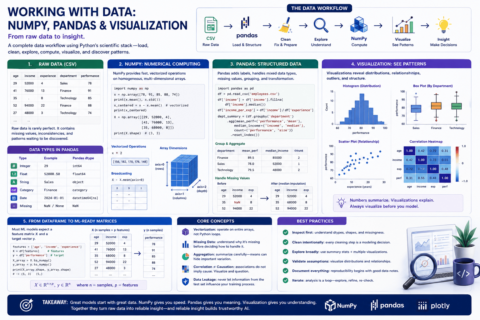
Introduction

Machine learning models ultimately learn from numbers. Whether the original information consists of customer transactions, scientific measurements, survey responses, medical observations, satellite imagery, or text embeddings, it must eventually be represented in computational structures that algorithms can process efficiently.

This makes data engineering and numerical reasoning foundational AI skills. Before training a model, practitioners must understand the shape of their data, identify missing or invalid observations, transform variables appropriately, detect unusual patterns, and determine whether the dataset actually contains information capable of answering the question being investigated.

Python's scientific ecosystem provides several complementary tools for this process. NumPy supplies efficient multidimensional numerical arrays and vectorized computation. Pandas builds higher-level labeled structures for working with heterogeneous tabular data. Visualization libraries such as Matplotlib and Plotly transform numerical patterns into graphical representations that humans can inspect far more efficiently than thousands of rows in a table.

The important skill is not memorizing library functions. It is understanding how these tools participate in a coherent analytical workflow:

CSV → Pandas → Clean → Explore → NumPy Operations → Visualize → Insight

From Raw Data to Computational Representation

A CSV file appears simple because humans see rows and columns. Computationally, however, those columns may represent very different kinds of information. Age may be an integer, income a continuous measurement, employment status a categorical variable, a timestamp a temporal value, and a missing observation something requiring explicit representation.

Consider a small dataset:

age,income,experience,department,performance
29,52000,4,Sales,78
41,76000,13,Finance,91
35,,8,Technology,85
52,94000,22,Finance,88
27,48000,3,Technology,74

Pandas can load this into a DataFrame:

import pandas as pd

df = pd.read_csv("employees.csv")

print(df.head())
print(df.info())

The first command shows observations. The second tells us something arguably more important: how Pandas has interpreted the structure.

An experienced analyst does not immediately begin calculating statistics. The first questions are structural: How many observations are present? What does one row represent? Which columns are numeric? Which are categorical? Are values missing? Are the inferred data types appropriate?

That examination establishes the analytical meaning of the dataset before transformations begin.

NumPy: The Numerical Layer Beneath the Workflow

At the foundation of much of Python's scientific computing ecosystem is NumPy, whose central abstraction is the ndarray: an efficient, homogeneous, multidimensional array.

A simple array can be created as follows:

import numpy as np

scores = np.array([78, 91, 85, 88, 74])

print(scores)
print(scores.shape)
print(scores.dtype)

Unlike an ordinary Python list, a NumPy array is designed specifically for numerical computation. Its elements typically share a common data type and are arranged in memory in ways that allow operations to be performed efficiently.

The distinction becomes important when working with thousands or millions of values. Rather than repeatedly processing individual elements in Python, NumPy performs many calculations using optimized low-level routines.

For example:

scores.mean()
scores.std()
scores.min()
scores.max()

More importantly, operations can be applied across an entire array:

centered = scores - scores.mean()

Conceptually, this subtracts the mean from every observation:

This is an example of vectorized computation. Instead of describing how to process each individual value, we describe the mathematical transformation to perform on the entire structure.

That shift, from thinking in loops to thinking in arrays, is one of the most important transitions in scientific Python.

Shape, Dimensions, and Axes

Understanding shape becomes increasingly important as data moves from conventional analysis into machine learning and deep learning.

Consider:

X = np.array([
    [29, 52000, 4],
    [41, 76000, 13],
    [35, 68000, 8],
    [52, 94000, 22]
])

print(X.shape)

The result is:

(4, 3)

This tells us that the array contains four observations and three features.

In conventional machine learning, a feature matrix is often represented as:

where n represents the number of observations and p represents the number of features.

This notation becomes extremely important later. A grayscale image might be represented as a two-dimensional matrix, a color image as a three-dimensional array, and a batch of images as a four-dimensional tensor. Large Language Models similarly operate on tensors containing batches, token sequences, embeddings, attention values, and model parameters.

NumPy therefore introduces much more than a convenient array library. It teaches the dimensional way of thinking that underlies modern AI.

Broadcasting: Powerful but Worth Understanding

NumPy's broadcasting system allows operations between arrays of compatible but different shapes.

Suppose we have:

X = np.array([
    [10, 100],
    [20, 200],
    [30, 300]
])

means = X.mean(axis=0)

centered = X - means

means has one value for each column, while X contains several rows. NumPy automatically applies the corresponding column mean across every observation.

This makes mathematical code concise, but it can also produce subtle errors when dimensions happen to be compatible even though the analyst intended something else. Advanced NumPy work therefore requires constant awareness of shape.

A useful debugging habit is simple:

print(X.shape)
print(means.shape)
print(centered.shape)

When working with AI models, many apparent algorithmic problems are actually shape problems.

Pandas: Adding Meaning to Arrays

NumPy arrays are excellent for numerical computation, but real-world datasets are rarely homogeneous numerical matrices.

A table might simultaneously contain numbers, strings, dates, categories, missing values, and identifiers. Pandas provides higher-level abstractions designed for exactly this situation.

Its two central structures are the Series, representing a labeled one-dimensional sequence, and the DataFrame, representing a labeled two-dimensional table.

df = pd.read_csv("employees.csv")

print(df.shape)
print(df.columns)
print(df.dtypes)

Unlike a plain numerical matrix, the DataFrame preserves semantic information through column names and indices. This allows transformations to be expressed in terms of variables rather than numerical positions:

df["income"].mean()

instead of something like:

X[:, 1].mean()

Neither representation is universally superior. Pandas is generally more convenient while understanding and transforming heterogeneous datasets; NumPy becomes valuable when the task moves toward efficient numerical operations.

Professional data workflows frequently move between both.

Cleaning Data Is a Modeling Decision

Data cleaning is sometimes described as mechanical housekeeping: remove missing values, fix duplicates, correct types, and continue.

In reality, cleaning decisions can fundamentally alter the statistical meaning of a dataset.

Consider the missing income value in our example:

df.isna().sum()

One possible response is to remove every incomplete row:

df_clean = df.dropna()

Another is to replace missing income with the median:

df["income"] = df["income"].fillna(df["income"].median())

These operations are technically simple but conceptually very different. Removing observations changes the sample. Imputation introduces estimated values. If missingness is systematically related to the phenomenon being studied, either approach may introduce bias.

The correct question is therefore not:

"Which Pandas function removes missing values?"

It is:

"Why are these values missing, and what assumptions am I making when I decide how to handle them?"

Filtering, Selecting, and Transforming

A major part of analytical work consists of selecting subsets of observations and creating meaningful transformations.

For example:

experienced = df[df["experience"] >= 10]

Multiple conditions can be combined:

subset = df[
    (df["experience"] >= 10) &
    (df["performance"] >= 85)
]

New variables can also be derived from existing ones:

df["income_per_year_experience"] = (
    df["income"] / df["experience"]
)

The ability to construct variables is especially important in machine learning, where feature engineering can strongly influence model performance.

However, every engineered feature encodes assumptions. Dividing income by years of experience may appear mathematically reasonable, but whether the resulting variable has meaningful interpretation depends on the research question and data-generating process.

Good data science therefore combines computational skill with domain reasoning.

Grouping and Aggregation

Individual observations often become more informative when analyzed in groups.

Suppose we want average performance by department:

department_summary = (
    df.groupby("department")
    .agg(
        mean_performance=("performance", "mean"),
        median_income=("income", "median"),
        employees=("performance", "size")
    )
    .reset_index()
)

print(department_summary)

This transformation moves the analysis from the individual level to the group level.

Aggregation is enormously powerful, but it can also conceal variation. Two departments with identical average performance may have dramatically different distributions. One might contain employees clustered tightly around the mean, while another contains both very high and very low performers.

This is one reason visualization becomes essential.

Visualization & Interactive Data Exploration

Visualization: Seeing What Summary Statistics Hide

Consider two datasets with the same mean and similar standard deviation. Their numerical summaries might suggest that they behave similarly, yet one could be approximately normal while another contains extreme outliers, multiple clusters, or nonlinear patterns.

Visualization allows analysts to inspect the shape of the data rather than relying solely on numerical summaries.

A histogram provides an initial view of a quantitative distribution:

import matplotlib.pyplot as plt

df["performance"].plot(
    kind="hist",
    bins=10,
    edgecolor="black"
)

plt.xlabel("Performance Score")
plt.ylabel("Frequency")
plt.title("Distribution of Performance Scores")
plt.show()

A boxplot can reveal spread and potential outliers:

df.boxplot(column="performance", by="department")

plt.suptitle("")
plt.title("Performance by Department")
plt.ylabel("Performance Score")
plt.show()

And a scatter plot can reveal relationships between quantitative variables:

df.plot.scatter(
    x="experience",
    y="performance"
)

plt.title("Experience and Performance")
plt.show()

The purpose of these plots is not decoration. Each visualization asks a different analytical question.

A histogram asks, "What does the distribution look like?"

A boxplot asks, "How do distributions differ across groups?"

A scatter plot asks, "How do two quantitative variables vary together?"

Interactive Visualization with Plotly

Static visualizations remain invaluable for analysis and publication, but interactive visualization becomes useful when datasets contain many dimensions or when users need to explore individual observations.

Plotly provides interactive charts within Python:

import plotly.express as px

fig = px.scatter(
    df,
    x="experience",
    y="performance",
    color="department",
    hover_data=["age", "income"]
)

fig.show()

The underlying analytical question remains similar to the Matplotlib scatter plot, but the user can now inspect individual points, zoom into regions, hide categories, and explore additional variables through interaction.

This distinction suggests an important design principle: static graphics are often ideal for communicating a carefully selected analytical finding, while interactive graphics are particularly valuable for exploration.

Correlation Is a Starting Point, Not a Conclusion

Once several quantitative variables are available, analysts often calculate correlations:

numeric = df.select_dtypes(include="number")

correlations = numeric.corr()

print(correlations)

For two variables X and Y, Pearson's correlation coefficient can be written as:

Values near $1$ indicate strong positive linear association, values near $-1$ indicate strong negative linear association, and values near zero indicate little linear association.

The final word matters.

A near-zero Pearson correlation does not prove that two variables are unrelated. They may have a strong nonlinear relationship. Outliers may also substantially alter the coefficient.

This is another reason numerical analysis and visualization should work together rather than independently.

From DataFrames to Machine Learning Matrices & Data Leakage

Eventually, an exploratory dataset must become something a machine learning algorithm can consume.

Suppose performance is our target variable and several numerical columns are predictors:

features = [
    "age",
    "income",
    "experience"
]

X = df[features]
y = df["performance"]

Here we have created the two structures that appear throughout supervised machine learning:

and

Their dimensions can be inspected:

print(X.shape)
print(y.shape)

At this point, Pandas structures may be passed directly to many machine learning libraries or converted to NumPy arrays:

X_array = X.to_numpy()
y_array = y.to_numpy()

The workflow has therefore moved full circle. Raw tabular information entered through Pandas, was cleaned and explored semantically, and can now become the numerical representation required for modeling.

Data Leakage: When Preparation Accidentally Reveals the Answer

One of the most serious mistakes in machine learning occurs when information from outside the legitimate training process influences the model.

This is known as data leakage.

Imagine standardizing an entire dataset before separating training and test observations. The mean and standard deviation used for transformation would then contain information from the test data.

The transformation itself may seem harmless:

X_scaled = (
    X - X.mean()
) / X.std()

Mathematically, this performs standardization:

But if $\mu$ and $\sigma$ were calculated using observations that are supposed to remain unseen during training, information has crossed the boundary between training and evaluation.

The correct machine learning workflow generally determines preprocessing parameters using the training data only, then applies those learned transformations to validation or test data.

This illustrates a broader lesson: even perfectly correct NumPy or Pandas code can produce scientifically invalid results if the analytical workflow is poorly designed.

A Compact End-to-End Exploration

We can now combine the major ideas into a small exploratory workflow:

import pandas as pd
import matplotlib.pyplot as plt

# Load
df = pd.read_csv("employees.csv")

# Inspect
print(df.info())
print(df.describe(include="all"))

# Missingness
print(df.isna().sum())

# Clean
df["income"] = df["income"].fillna(
    df["income"].median()
)

# Explore groups
print(
    df.groupby("department")["performance"]
    .agg(["mean", "median", "std", "count"])
)

# Visualize distribution
df["performance"].plot(
    kind="hist",
    bins=10,
    edgecolor="black"
)

plt.xlabel("Performance")
plt.show()

# Prepare possible model inputs
X = df[["age", "income", "experience"]]
y = df["performance"]

print("Features:", X.shape)
print("Target:", y.shape)

The code is intentionally uncomplicated. The sophistication lies in understanding why each step occurs and what assumptions it introduces.

That distinction separates merely manipulating data from conducting an analysis.

From Data to Insight

The complete workflow can now be understood as a sequence of transformations:

CSV → Pandas → Clean → Explore → NumPy Operations → Visualize → Insight

Yet the arrows conceal an important reality: real analysis is rarely perfectly linear. A visualization may reveal an error that sends us back to cleaning. A group comparison may reveal that a variable was incorrectly encoded. An unexpected distribution may require examining the original data source. A modeling result may force us to reconsider feature construction.

Professional data analysis is therefore better understood as an iterative reasoning process.

Tools such as NumPy and Pandas make transformations computationally efficient, while visualization allows humans to interrogate their consequences. Neither replaces statistical reasoning, domain expertise, or critical judgment.

The objective is not merely to produce a clean table.

It is to construct a defensible representation of reality from which reliable conclusions—and eventually reliable models—can be developed.

Conclusion

NumPy, Pandas, and visualization libraries occupy different layers of the modern AI data stack. NumPy provides efficient numerical structures and vectorized operations. Pandas adds labels, heterogeneous data types, grouping, transformation, and powerful tabular semantics. Visualization converts distributions and relationships into forms that human perception can examine rapidly.

Together, these tools transform raw observations into computationally meaningful data.

But proficiency involves more than knowing their APIs. Advanced practitioners must understand dimensionality, data types, missingness, aggregation, feature construction, statistical relationships, leakage, and the assumptions introduced by every transformation.

This is why data preparation sits at the foundation of machine learning rather than merely preceding it.

In the next article, Building Your First Machine Learning Workflow, we will take the feature matrix X and target vector y created here and move into the full modeling lifecycle: splitting data, preprocessing features, training models, generating predictions, evaluating generalization, and constructing reproducible machine learning pipelines.

Key Takeaways

• NumPy provides the multidimensional numerical array foundation underlying much of scientific Python and modern AI.
• Vectorized computation allows mathematical transformations to operate efficiently across entire arrays rather than through explicit Python loops.
• Understanding shape, dimensions, axes, and broadcasting prepares learners for tensors and deep learning.
• Pandas DataFrames add semantic structure to heterogeneous tabular data through labels, indices, data types, grouping, and transformation.
• Data cleaning is not merely technical housekeeping; every cleaning decision introduces analytical assumptions.
• Visualization reveals distributions, relationships, clusters, outliers, and nonlinear patterns that summary statistics may conceal.
• Matplotlib is particularly useful for controlled static analysis, while Plotly supports interactive exploration.
• Correlation measures particular forms of association and should generally be interpreted alongside visualization.
• Machine learning commonly represents predictors as a feature matrix $ and outcomes as a target vector $.
• Data leakage can make a technically correct analysis scientifically invalid by allowing information from evaluation data to influence training.
• Responsible AI begins with understanding the quality, meaning, provenance, and limitations of the data from which models learn.