Module 7: Correlation & Regression

Introduction

Modules 5 and 6 focused on hypothesis testing and group comparisons. The t-tests evaluated differences involving one or two means, while ANOVA extended this framework to several groups and factorial designs by partitioning variation into systematic and residual components. Module 7 moves from comparing means to modelling relationships among variables. The central question is no longer only whether groups differ, but whether an outcome changes systematically as one or more predictors change, how much variation the model explains, and how accurately the model predicts new or observed outcomes.

Regression distinguishes between a dependent variable, which represents the outcome being modelled, and one or more predictor variables, which are used to explain or predict variation in that outcome. In an explanatory analysis, the primary objective is to estimate and interpret relationships, assess statistical evidence, and determine the contribution of each predictor while holding the others constant. In a predictive analysis, greater emphasis is placed on how well the fitted model generates accurate predictions or classifications. These objectives overlap, but they are not identical: a statistically significant predictor does not automatically produce strong predictive performance, and a useful predictive model may contain relationships that require cautious substantive interpretation.

This module begins with correlation as a concise description of bivariate association and then develops simple and multiple linear regression. It introduces fitted values, residuals, model fit, coefficient interpretation, diagnostics, multicollinearity, and binary predictor coding. The final sections extend the modelling framework to binary logistic regression, where predicted probabilities are converted into classifications and evaluated using confusion-matrix measures and ROC analysis. This progression marks an important transition from individual hypothesis tests toward the broader statistical modelling principles used throughout data science and machine learning.

Learning Objectives

By the end of this module, you should be able to:

• Interpret scatterplots and Pearson's correlation coefficient in terms of direction, strength, statistical significance, and shared variance.
• Distinguish correlation from causation and identify conditions that can distort a bivariate association.
• Specify and interpret a simple linear regression model using an intercept, slope, fitted values, and residuals.
• Explain the least-squares criterion and the role of residual variation in model estimation.
• Interpret \(R\), \(R^2\), adjusted \(R^2\), the model F-test, and individual coefficient t-tests.
• Assess regression assumptions using residual-versus-fitted plots, Q–Q plots, the Shapiro–Wilk test, and the Durbin–Watson statistic.
• Distinguish outliers, high-leverage observations, and influential observations, and explain the purpose of Cook's distance.
• Interpret multiple regression coefficients while holding the other predictors constant.
• Distinguish unstandardised coefficients \(B\) from standardised coefficients \(\beta\).
• Evaluate multicollinearity using tolerance and variance inflation factors.
• Incorporate and interpret binary categorical predictors using dummy coding and reference categories.
• Explain why ordinary linear regression is unsuitable for binary outcomes.
• Interpret logistic regression coefficients, log odds, probabilities, Wald tests, and odds ratios.
• Evaluate logistic model fit using log-likelihood, AIC, pseudo-\(R^2\), and the Hosmer–Lemeshow test.
• Interpret classification thresholds, confusion matrices, accuracy, sensitivity, specificity, precision, and F1-score.
• Explain how ROC curves and AUC evaluate classification performance across thresholds.
• Distinguish statistical inference from predictive performance.
• Select appropriately among correlation, simple linear regression, multiple linear regression, and binary logistic regression.
• Use the LearnerBox Statistical Explorer to examine model fit, coefficients, diagnostics, probabilities, and classification performance.
• Interpret regression results numerically, statistically, practically, and in APA style.

LearnerBox Statistical Explorer

Correlation and Bivariate Association

Correlation describes the direction and strength of association between two variables. For two quantitative variables, the analysis should begin with a scatterplot. The scatterplot reveals whether the variables tend to increase or decrease together, whether the relationship is approximately linear, and whether unusual observations may influence the association. A correlation coefficient should therefore be interpreted alongside the observed pattern of data rather than as an isolated numerical result.

The statistical basis of correlation is covariance. Covariance indicates whether two variables vary together. A positive covariance occurs when values above the mean of one variable tend to occur with values above the mean of the other; a negative covariance occurs when higher values of one variable tend to occur with lower values of the other. Sample covariance is calculated as:

The magnitude of covariance depends on the measurement units of the variables, which makes direct comparison difficult. Pearson's product–moment correlation coefficient, denoted by \(r\), standardises covariance using the standard deviations of the two variables:

Because the covariance is standardised, Pearson's \(r\) ranges from \(-1\) to \(+1\). The sign indicates the direction of the association. A positive value indicates that higher values of one variable tend to accompany higher values of the other, whereas a negative value indicates that higher values of one variable tend to accompany lower values of the other. The absolute magnitude of \(r\) indicates the strength of the linear association. Values closer to \(0\) indicate weaker linear relationships, while values closer to \(1\) in absolute magnitude indicate stronger relationships.

Conventional guidelines sometimes describe absolute correlations of approximately .10, .30, and .50 as small, moderate, and large, respectively. These thresholds should be treated as general reference points rather than universal rules. The practical importance of a correlation depends on the research context, measurement quality, sample characteristics, and consequences of the relationship being studied.

The squared correlation coefficient, \(r^2\), is the coefficient of determination in the simple bivariate setting. It represents the proportion of variation shared through the linear relationship between the two variables. For example, if:

then:

The two variables share approximately 25% of their variation in the linear association. As shown later, this quantity has a direct relationship with \(R^2\) in simple linear regression with one predictor and an intercept.

Statistical inference for Pearson's correlation evaluates the null hypothesis that the population correlation is zero:

for a two-tailed test. A statistically significant result indicates evidence of a non-zero linear association in the population. The significance of \(r\), however, depends partly on sample size. In a large sample, a weak correlation may be statistically significant, whereas a stronger observed correlation in a small sample may not reach the selected significance level. The magnitude and practical meaning of \(r\) should therefore be interpreted together with its p-value.

Pearson's correlation is most appropriate when both variables are quantitative, observations are independent, and the relationship is approximately linear. The scatterplot should also be examined for influential unusual observations because Pearson's \(r\) can be sensitive to extreme values. Bivariate normality is relevant to the classical significance test and confidence interval for the population correlation, although visual inspection of the relationship remains essential. When variables are ordinal, the relationship is monotonic rather than linear, or the data structure is unsuitable for Pearson's correlation, a rank-based measure such as Spearman's \(\rho\) may be more appropriate.

Correlation provides a concise summary of bivariate association, but it does not specify an equation for predicting one variable from another. Once a systematic relationship has been identified, the next question is whether the value of an outcome can be modelled as a function of a predictor. This is the role of regression analysis.

Worked Example 7.1 — Correlation Between Age and Annual Income

1. Research Question

Is there a statistically significant linear association between Age and Annual Income among customers?

2. Variables

The analysis includes two quantitative variables:

• Age — customer age measured in years.
• Annual Income — annual customer income.

Neither variable is designated as a dependent variable for the correlation analysis. The objective is to quantify the linear association between them.

3. Hypotheses

A two-tailed Pearson correlation test is used because the research question asks whether an association exists without specifying its direction in advance.

\[ H_0:\rho=0 \] \[ H_1:\rho\neq0 \]

The significance level is:

\[ \alpha=.05 \]

4. Assumptions and Testing

Pearson's correlation requires quantitative variables, independent observations, an approximately linear relationship, and the absence of influential extreme observations that substantially distort the association. The classical significance test also assumes bivariate normality.

Both Age and Annual Income are quantitative variables, and each row in the dataset represents a separate customer. The independence requirement is therefore reasonable based on the dataset structure.

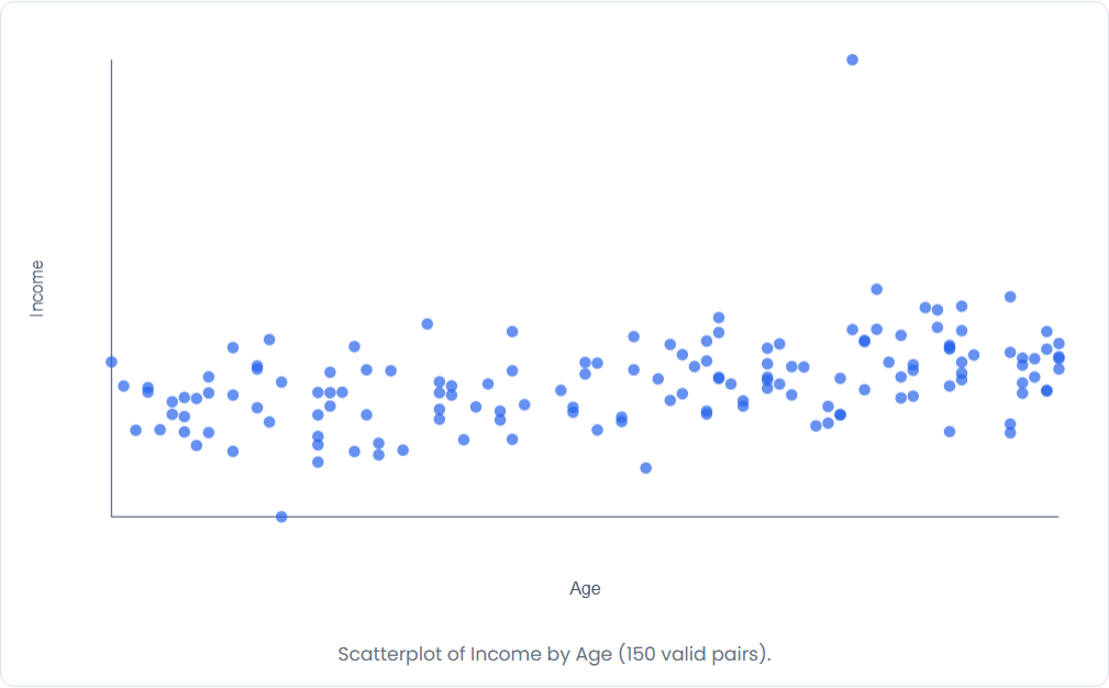
The scatterplot in Figure 7.1 shows a generally positive linear pattern: Annual Income tends to increase as Age increases. The relationship does not display a clear curved form. However, one customer has an unusually high Annual Income relative to the remainder of the sample. This observation should be noted because Pearson's \(r\) is sensitive to influential unusual observations.

The scatterplot therefore supports the use of Pearson's correlation for the present analysis, while the unusual high-income observation should be considered when interpreting the magnitude of the association.

5. Formula

Pearson's product–moment correlation coefficient is calculated as:

\[ r= \frac{\sum_{i=1}^{n}(x_i-\bar{x})(y_i-\bar{y})} {\sqrt{\sum_{i=1}^{n}(x_i-\bar{x})^2 \sum_{i=1}^{n}(y_i-\bar{y})^2}} \]

The coefficient standardises the degree to which Age and Annual Income vary together.

6. Manual Calculation

The complete row-by-row calculation is unnecessary because the dataset contains 150 observations. The key derived quantity for interpretation is the squared correlation:

\[ r^2=(.403)^2 \] \[ r^2=.1624 \]

Thus, Age and Annual Income share approximately 16.24% of their variation through the observed linear association.

7. LearnerBox Statistical Explorer

In the LearnerBox Dataset Viewer, select Scatterplot as the chart type, Age as the X variable, and Annual Income as the Y variable. The graph displays 150 valid pairs.

The statistical analysis gives:

\[ r=.403,\quad p<.001 \]

Figure 7.1 should be examined together with the numerical correlation. The upward pattern of observations is consistent with the positive value of \(r\), while the dispersion around the general trend indicates that the relationship is not perfect.

8. Four Layers of Interpretation

Numerical Result

The Pearson correlation between Age and Annual Income is:

\[ r=.403 \]

The positive sign indicates a positive association, and the magnitude indicates a moderately strong to strong linear relationship. The corresponding squared correlation is:

\[ r^2=.162 \]

Approximately 16.2% of the variation is shared through the linear association between Age and Annual Income.

Statistical Interpretation

The correlation is statistically significant:

\[ p<.001 \]

Because the p-value is below the significance level of .05, the null hypothesis is rejected. The sample provides strong statistical evidence of a positive linear association between Age and Annual Income.

Practical Interpretation

Older customers in this dataset tend to have higher Annual Incomes. The association is sufficiently substantial to be practically noticeable, although Age alone does not account for most of the variation in income. Approximately 73.5% of the variation is not shared through this bivariate linear relationship and may reflect other variables, random variation, measurement characteristics, or more complex relationships.

The result should not be interpreted causally. The analysis does not demonstrate that increasing a person's age causes Annual Income to increase. Age may be associated with career stage, experience, occupation, education, or other variables that contribute to income differences.

📝APA Result:A Pearson product–moment correlation showed a statistically significant positive association between Age and Annual Income, r(148) = .403, p < .001. Age and Annual Income shared approximately 16.2% of their variation.

9. Key Learning Point

A correlation of \(r=.403\) establishes a statistically significant positive linear association, but it does not provide a prediction equation or estimate how much Annual Income is expected to change for each additional year of Age. To answer those questions, the relationship must be expressed as a regression model.

Practice Exercises

Use the concepts from Worked Example 7.1 to answer the following questions.

Practice Exercise 1

A researcher reports a correlation of \(r=-.62\) between delivery time and customer satisfaction, with \(p<.001\). Interpret the direction, strength, and statistical significance of the relationship. Calculate and interpret \(r^2\).

Practice Exercise 2

A sample of 250 customers produces a correlation of \(r=.14\) between website visit duration and purchase amount, with \(p=.027\). A student concludes that the two variables have a strong relationship because the result is statistically significant. Evaluate this conclusion.

Practice Exercise 3

A scatterplot shows a clear U-shaped relationship between advertising frequency and customer engagement. Pearson's correlation is \(r=.03\), with \(p=.71\). Should the researcher conclude that advertising frequency and customer engagement are unrelated?

Simple Linear Regression

Simple linear regression models the relationship between one quantitative outcome variable and one predictor variable. Unlike correlation, which summarises the direction and strength of a symmetric association, regression assigns distinct roles to the variables. The predictor \(X\) is used to explain or predict variation in the outcome \(Y\).

The population regression model is:

where \(\beta_0\) is the population intercept, \(\beta_1\) is the population slope, and \(\varepsilon_i\) represents the error component for observation \(i\). The fitted sample regression equation is:

The fitted equation defines the regression line. For each value of \(X\), the line provides an estimated or fitted value of the outcome, denoted by \(\hat{Y}\).

Intercept and Slope

The intercept, \(b_0\), is the predicted value of \(Y\) when \(X=0\). Its substantive interpretation depends on whether zero is meaningful and within a reasonable range of the predictor. An intercept remains mathematically necessary for the model even when \(X=0\) has little practical relevance.

The slope, \(b_1\), represents the expected change in the predicted outcome for a one-unit increase in the predictor:

A positive slope indicates that predicted \(Y\) increases as \(X\) increases. A negative slope indicates that predicted \(Y\) decreases as \(X\) increases. The magnitude of \(b_1\) is interpreted in the original measurement units of the variables.

For example, if the fitted model is:

the slope indicates that each additional year of Age is associated with an expected increase of 950 units in predicted Annual Income. This is an association estimated by the model and should not automatically be interpreted as a causal effect.

Fitted Values and Residuals

Regression separates each observed outcome into a fitted component and a residual component:

The residual is the difference between the observed and fitted outcome:

A positive residual indicates that the observed value lies above the regression line; a negative residual indicates that it lies below the line. A residual of zero indicates that the fitted model predicts the observed outcome exactly for that case.

Residuals represent the variation in the outcome that remains after the fitted linear relationship with the predictor has been estimated. Their magnitude and pattern are therefore central to evaluating model fit and regression assumptions.

Least-Squares Estimation

Many possible straight lines could be drawn through a scatterplot. Ordinary least squares regression selects the intercept and slope that minimise the sum of squared residuals:

Squaring the residuals prevents positive and negative errors from cancelling and gives greater weight to larger prediction errors. The fitted regression line is therefore the line that produces the smallest possible SSE among all lines represented by the linear model.

For simple linear regression, the estimated slope can be expressed as:

and the intercept is:

The fitted regression line therefore passes through the point \((\bar{x},\bar{y})\).

Explained and Residual Variation

The variance-partitioning logic introduced in ANOVA continues directly into regression. Total variation in the outcome is partitioned into variation explained by the regression model and unexplained residual variation:

The total sum of squares is:

The regression sum of squares measures variation in the fitted values around the outcome mean:

The error sum of squares measures residual variation:

Regression is therefore not conceptually separate from ANOVA. Both procedures evaluate systematic variation relative to residual variation. The difference lies in how the systematic component is specified by the statistical model.

R and the Coefficient of Determination

In simple linear regression, \(R\) describes the correlation between the observed outcome values and the values predicted by the regression model. With one predictor and an intercept, its magnitude corresponds to the absolute value of the Pearson correlation between \(X\) and \(Y\).

The coefficient of determination, \(R^2\), is the proportion of total outcome variation explained by the fitted regression model:

Equivalently:

For simple linear regression with one predictor and an intercept:

Thus, the correlation result from Worked Example 7.1:

corresponds to:

A regression model using Age as the sole predictor therefore explains approximately 16.2% of the observed variation in Annual Income.

Adjusted R²

The adjusted coefficient of determination modifies \(R^2\) for sample size and the number of predictors in the model:

where \(n\) is the sample size and \(p\) is the number of predictors.

Unlike \(R^2\), adjusted \(R^2\) includes a penalty for model complexity. Its importance becomes greater in multiple regression, where additional predictors may increase \(R^2\) even when they contribute little useful explanatory information. In simple regression, \(R^2\) and adjusted \(R^2\) are usually close.

The Model F-Test

The regression F-test evaluates the statistical significance of the model as a whole. For simple linear regression, the hypotheses are:

The F statistic compares the regression mean square with the residual mean square:

A statistically significant F-test indicates that the fitted regression model explains more outcome variation than would be expected under the null hypothesis that the predictor has no linear contribution to the model.

With one predictor:

and:

The model is reported using the F statistic, its two degrees of freedom, and the p-value.

The Coefficient t-Test

Each regression coefficient can also be evaluated individually. For the slope:

The t statistic is:

A statistically significant coefficient test indicates that the estimated slope differs from zero after accounting for its sampling uncertainty.

In simple linear regression, the model F-test and the slope t-test evaluate the same single-predictor null hypothesis. Consequently:

and the two tests produce the same non-directional inferential conclusion. This equivalence changes conceptually in multiple regression: the F-test evaluates the predictors jointly, whereas each coefficient t-test evaluates one predictor while holding the other predictors constant.

Simple linear regression therefore extends correlation from a measure of association to an explicit statistical model. The fitted equation estimates the expected outcome at a given predictor value, \(R^2\) quantifies explained variation, and inferential tests evaluate whether the observed linear relationship is supported statistically. The next worked example applies this framework to Age and Annual Income.

Worked Example 7.2 — Predicting Annual Income from Age

1. Research Question

Does Age significantly predict Annual Income among customers, and how much variation in Annual Income is explained by the fitted linear regression model?

2. Variables

The analysis contains one quantitative outcome variable and one quantitative predictor:

• Outcome variable: Annual Income
• Predictor variable: Age

The model treats Age as the predictor \(X\) and Annual Income as the outcome \(Y\). The objective is to estimate the expected change in Annual Income associated with a one-year increase in Age.

3. Hypotheses

The model evaluates whether the population slope for Age differs from zero:

\[ H_0:\beta_1=0 \] \[ H_1:\beta_1\neq0 \]

The significance level is:

\[ \alpha=.05 \]

Under the null hypothesis, Age has no linear predictive contribution to Annual Income. The alternative hypothesis states that the population slope is non-zero.

4. Assumptions and Testing

The analysis uses quantitative outcome and predictor variables. Each row represents a separate customer, so independence between observations is reasonable from the dataset structure.

The relationship between Age and Annual Income is approximately linear, making a simple linear regression model appropriate. Scatterplots and residual plots should always be examined for evidence of curvature, changing variance, or influential observations.

Residual normality was assessed using the Shapiro–Wilk test. For this model:

\[ W=0.842,\quad p<.0001 \]

The statistically significant result indicates evidence against residual normality. Consequently, the residual Q–Q plot and any unusually influential observations should be examined alongside the formal test rather than relying solely on the p-value.

The Durbin–Watson statistic is:

\[ DW=1.919 \]

A value close to 2 indicates little evidence of first-order residual autocorrelation. The independence of residual errors therefore appears reasonable.

📋Remember: Regression assumptions should always be evaluated using the residual structure of the fitted model. A statistically significant Shapiro–Wilk test does not automatically invalidate the regression model; it should be interpreted together with the Q–Q plot, residual plot, sample size, and any unusual observations.

5. Formula

The simple linear regression model is:

\[ Y_i=\beta_0+\beta_1X_i+\varepsilon_i \]

For the present analysis:

\[ \text{Income}_i = \beta_0 + \beta_1(\text{Age}_i) + \varepsilon_i \]

The fitted regression equation is:

\[ \widehat{\text{Income}} = b_0+b_1(\text{Age}) \]

Using the estimated coefficients:

\[ \widehat{\text{Income}} = 78{,}693.646 + 296.637(\text{Age}) \]

6. Manual Calculation

The estimated slope for Age is:

\[ b_1=296.637 \]

Its standard error is:

\[ SE(b_1)=55.361 \]

The coefficient t statistic is calculated as:

\[ t= \frac{b_1}{SE(b_1)} \] \[ t= \frac{296.637}{55.361} = 5.358 \]

Because the model contains one predictor:

\[ df=n-2 \] \[ df=150-2=148 \]

The resulting coefficient test is:

\[ t(148)=5.358,\quad p<.0001 \]

The model F statistic is:

\[ F(1,148)=28.710,\quad p<.0001 \]

For a simple linear regression containing one predictor:

\[ F=t^2 \]

Therefore:

\[ 5.358^2\approx28.710 \]

The model F-test and the Age coefficient t-test therefore produce the same inferential conclusion.

The coefficient of determination is:

\[ R^2=.162 \]

Therefore:

\[ .162\times100=16.2\% \]

The model explains approximately 16.2% of the observed variation in Annual Income.

7. LearnerBox Statistical Explorer

In the Regression tab, select Income as the dependent variable and Age as the predictor. The Explorer reports the model summary, regression diagnostics, fitted relationship, and regression coefficients.

The model summary gives:

\[ R=.403 \] \[ R^2=.162 \] \[ \text{Adjusted }R^2=.157 \]

The residual standard error is:

\[ 16{,}084.062 \]

The overall regression model is statistically significant:

\[ F(1,148)=28.710,\quad p<.0001 \]

The coefficients table reports the estimated intercept and Age coefficient together with their standard errors, t statistics, and p-values:

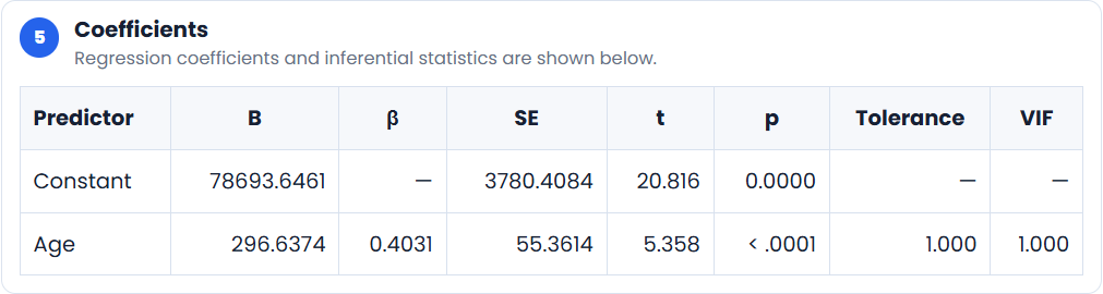
Figure 7.2 shows the estimated intercept and Age coefficient together with their standard errors, test statistics, and p-values.

The unstandardised Age coefficient is:

\[ B=296.637 \]

This coefficient is positive and statistically significant:

\[ t(148)=5.358,\quad p<.0001 \]

The coefficient indicates that, for every additional year of Age, predicted Annual Income increases by approximately $296.64, on average.

The intercept is:

\[ B_0=78{,}693.646 \]

Mathematically, this is the predicted Annual Income when Age equals zero. Because an age of zero lies outside the observed customer age range and has little substantive relevance, the intercept should not be given a practical interpretation.

The standardised coefficient for Age is:

\[ \beta=.403 \]

The positive standardized coefficient indicates a moderate positive relationship between Age and Annual Income.

8. Four Layers of Interpretation

Numerical Result

The fitted regression model is:

\[ \widehat{\text{Income}} = 78{,}693.646 + 296.637(\text{Age}) \]

The positive slope indicates that predicted Annual Income increases as Age increases. The model has \(R=.403\), \(R^2=.162\), and adjusted \(R^2=.157\). Approximately 16.2% of the observed variation in Annual Income is explained by Age.

Statistical Interpretation

The overall regression model is statistically significant:

\[ F(1,148)=28.710,\quad p<.0001 \]

The null hypothesis that the population slope equals zero is rejected. The Age coefficient is also statistically significant:

\[ B=296.637,\quad SE=55.361,\quad \beta=.403,\quad t(148)=5.358,\quad p<.0001 \]

The analysis therefore provides strong statistical evidence that Age is a positive predictor of Annual Income.

Residual normality was not supported by the Shapiro–Wilk test (\(W=0.842,\ p<.0001\)). Although this indicates some departure from normality, the regression results should be interpreted together with the residual plots and other diagnostic evidence rather than relying solely on the normality test.

Practical Interpretation

Each additional year of Age is associated with an average increase of approximately $297 in predicted Annual Income. Although Age provides statistically significant predictive information, it explains only 16.2% of the variability in Annual Income.

The remaining variation is associated with factors not included in this simple regression model together with residual variability. Variables such as education, employment status, occupation, work experience, and geographic region may substantially improve predictive performance.

As with all observational regression models, the results describe an association rather than a causal relationship. The estimated slope should therefore not be interpreted as evidence that increasing age directly causes higher annual income.

📝APA Result: A simple linear regression was conducted to examine whether Age predicted Annual Income. The regression model was statistically significant, F(1, 148) = 28.710, p < .001, \(R^2=.162\), adjusted \(R^2=.157\). Age was a statistically significant positive predictor of Annual Income, \(B=296.637\), \(SE=55.361\), \(\beta=.403\), t(148) = 5.358, p < .001. Each additional year of Age was associated with an estimated increase of approximately $296.64 in predicted Annual Income.

9. Key Learning Point

Simple linear regression extends correlation by expressing the relationship as a prediction equation:

The regression coefficient quantifies the expected change in the outcome associated with a one-unit increase in the predictor, while \(R^2\) indicates the proportion of outcome variability explained by the model. In this example, Age is a statistically significant predictor of Annual Income, although most of the variation remains unexplained by this single-predictor model.

Practice Exercise 7.1

A simple linear regression predicting examination score from weekly study hours produces the fitted equation:

Interpret the intercept and slope. Calculate the predicted examination score for a student who studies 8 hours per week.

Practice Exercise 7.2

A regression model reports:

Interpret the model fit and statistical significance.

Practice Exercise 7.3

A simple regression model produces the following coefficient result:

Interpret the coefficient and explain the relationship between the coefficient t-test and the model F-test.

Regression Assumptions and Model Diagnostics

Ordinary least squares regression estimates the coefficients that minimise squared residual error, but valid model interpretation requires examination of the assumptions underlying the fitted model. Regression diagnostics evaluate whether the specified functional form and residual structure are reasonably consistent with those assumptions and whether individual observations exert disproportionate influence on the estimated coefficients.

Diagnostics should not be treated as a sequence of automatic pass-or-fail tests. A statistically significant diagnostic test or an unusual point in a graph identifies a feature that requires investigation. The analyst must consider the magnitude and pattern of the departure, the sample size, the purpose of the model, and whether the substantive conclusions are sensitive to the issue.

Linearity

Linear regression assumes that the expected value of the outcome is a linear function of the predictors. In simple regression:

The assumption does not require every observation to lie close to a straight line. It requires the conditional mean structure to be appropriately represented by the linear model.

Linearity can initially be assessed using a scatterplot of the outcome against the predictor. After fitting the model, the residual-versus-fitted plot provides a more direct diagnostic. Residuals should be distributed around zero without systematic curvature. A U-shaped, inverted U-shaped, or other structured pattern suggests that the linear specification is failing to represent the relationship adequately.

When non-linearity is present, possible responses include transforming variables, adding polynomial or other non-linear terms, or fitting a model designed for the observed functional form. Simply reporting a significant linear coefficient does not establish that a straight-line model adequately represents the data.

Independence of Errors

Regression assumes that the errors associated with different observations are independent. Formally:

Independence is primarily a property of the research design and data structure. Repeated observations from the same participant, measurements clustered within organisations, and sequential time-series observations may produce correlated errors. Ordinary linear regression does not explicitly model such dependence.

For ordered observations, the Durbin–Watson statistic provides a diagnostic for first-order residual autocorrelation:

The statistic ranges approximately from 0 to 4. A value near 2 indicates little evidence of first-order autocorrelation. Values substantially below 2 suggest positive autocorrelation, whereas values substantially above 2 suggest negative autocorrelation.

The Durbin–Watson statistic should not replace knowledge of the sampling design. A value near 2 cannot establish independence when observations are known to be clustered or repeatedly measured. Such data may require multilevel, repeated-measures, or time-series models.

Homoscedasticity

The homoscedasticity assumption states that the conditional variance of the errors is constant across values of the predictors:

In practical terms, the vertical spread of residuals should remain reasonably stable across the range of fitted values. When residual variability systematically increases or decreases, the model exhibits heteroscedasticity.

The residual-versus-fitted plot is the primary graphical diagnostic. A roughly constant horizontal band of residuals around zero supports homoscedasticity. A funnel, cone, or fan-shaped pattern suggests changing residual variance.

Heteroscedasticity does not necessarily make the ordinary least squares coefficient estimates biased, but it can distort conventional standard errors, confidence intervals, and hypothesis tests. Depending on the analytical objective and source of the problem, possible responses include transformation, heteroscedasticity-consistent standard errors, weighted least squares, or an alternative model specification.

Residual Normality

Classical regression inference assumes that the model errors are normally distributed conditional on the predictors:

Normality is primarily relevant to the exact small-sample behaviour of coefficient tests and confidence intervals. Ordinary least squares estimation does not require the raw outcome or predictor variables themselves to be normally distributed.

Residual normality should be evaluated using the normal Q–Q plot together with an appropriate formal test such as the Shapiro–Wilk test. In a Q–Q plot, residual quantiles are compared with the theoretical quantiles expected under a normal distribution. Points that follow the reference line reasonably closely support approximate normality. Systematic curvature, asymmetric departures, or large deviations in the tails suggest non-normal residual behaviour.

The Shapiro–Wilk test evaluates:

A small p-value provides evidence against residual normality. However, formal normality tests are sensitive to sample size. Large samples may identify relatively minor departures, while small samples may have limited power to detect important non-normality. The Shapiro–Wilk result should therefore be interpreted alongside the Q–Q plot and the observed residual structure.

In Worked Example 7.2:

The test provides strong evidence against residual normality. The unusual high-income observation and departure visible in the diagnostic plots should therefore be investigated. The correct response is not to ignore the diagnostic result or automatically abandon the model, but to determine why the residual distribution departs from normality and whether the substantive conclusions are sensitive to that departure.

Outliers and Unusual Residuals

An outlier in the regression context is an observation with an outcome value that is unusual relative to the value predicted by the fitted model. Such an observation typically has a large residual:

Because raw residual magnitude depends on the scale of the outcome, standardised or studentised residuals are often used to identify unusually large prediction errors. Residuals beyond approximately \(\pm2\) merit attention, while values beyond approximately \(\pm3\) are commonly treated as particularly unusual. These are diagnostic guidelines rather than automatic deletion rules.

An outlier may represent a data-entry error, a measurement problem, a genuine extreme case, or evidence that the fitted model does not adequately represent part of the population. The observation should be investigated in context before any decision is made.

Leverage

A large residual is not the only way an observation can be unusual. Leverage describes how unusual an observation's predictor values are relative to the predictor distribution. In simple regression, an observation with an \(X\) value far from \(\bar{X}\) has greater potential to affect the position of the fitted regression line.

Leverage values are obtained from the diagonal elements of the regression hat matrix and are commonly denoted by:

The average leverage is:

where \(p\) is the number of predictors and the additional parameter represents the intercept. Values substantially larger than the average leverage, often assessed using guidelines such as:

or:

may warrant investigation.

High leverage does not automatically imply that an observation is problematic. A case may have unusual predictor values while still lying close to the fitted regression relationship. Leverage identifies the potential to influence the model, not the actual magnitude of influence.

Influential Observations and Cook's Distance

An influential observation is a case whose presence materially affects the fitted regression model. Removing an influential observation may noticeably alter the estimated coefficients, fitted values, or substantive interpretation.

The distinction among outliers, high-leverage observations, and influential observations is important:

• An outlier has an unusually large residual.
• A high-leverage observation has unusual predictor values.
• An influential observation materially changes the fitted model.

An observation is particularly capable of becoming influential when it combines substantial leverage with a large residual. Cook's distance, denoted by \(D_i\), summarises the influence of an observation by considering both its residual and leverage.

Conceptually:

Larger Cook's distance values indicate observations that have a greater effect on the fitted regression estimates. A frequently cited guideline is:

as a signal of potentially substantial influence. A more sensitive screening guideline is:

These values should be used as diagnostic flags rather than automatic exclusion criteria.

A Practical Diagnostic Workflow

Regression diagnostics are most effective when the different sources of evidence are considered together. After fitting a model, examine the residual-versus-fitted plot for curvature and changing variance. Inspect the normal Q–Q plot and Shapiro–Wilk result for residual normality. Consider the Durbin–Watson statistic when the ordering of observations makes residual autocorrelation relevant. Identify observations with unusually large residuals, examine high-leverage cases, and evaluate influence using Cook's distance when available.

The diagnostic process can be summarised as:

Fit the model → inspect residual patterns → assess residual distribution → examine dependence → identify unusual predictor values → evaluate influential observations → determine whether conclusions are robust.

Once the assumptions and residual structure of a regression model are understood, the modelling framework can be extended beyond a single predictor. Multiple linear regression estimates the relationship between an outcome and several predictors simultaneously, allowing the contribution of each predictor to be interpreted while holding the others constant.

Multiple Linear Regression

Multiple linear regression extends simple regression by modelling a continuous outcome using two or more predictors simultaneously. The population model is:

The fitted sample model is:

Each coefficient estimates the relationship between one predictor and the outcome while holding the other predictors constant. This is the defining interpretive feature of multiple regression. A coefficient therefore represents an adjusted effect: the estimated contribution of a predictor after accounting statistically for the other variables included in the model.

For example, a model predicting Annual Income from Age, Credit Score, and Purchase Amount may be written as:

The Age coefficient estimates the expected change in Annual Income associated with a one-year increase in Age while Credit Score and Purchase Amount are held constant. It should not be interpreted as the unadjusted bivariate relationship between Age and Annual Income.

Adjusted Effects and Predictor Overlap

Predictors in a multiple regression model may explain overlapping portions of outcome variation. Age and Credit Score, for example, may both be associated with Annual Income and may also be correlated with one another. The multiple regression coefficients separate their contributions statistically by estimating the association between each predictor and the outcome after accounting for the remaining predictors.

As a result, a predictor that has a statistically significant bivariate correlation with the outcome may become non-significant in a multiple regression model. This can occur when its association with the outcome is largely shared with another predictor. Conversely, a predictor's adjusted relationship may become clearer after another source of variation is controlled.

The coefficient \(b_j\) can be interpreted as the expected difference in the predicted outcome associated with a one-unit difference in \(X_j\), conditional on equal values of the other predictors:

This interpretation is statistical rather than necessarily causal. Including additional predictors does not automatically eliminate confounding or establish that the estimated coefficient represents a causal effect.

Unstandardised Coefficients B

The unstandardised regression coefficient, commonly labelled \(B\), is expressed in the original units of the predictor and outcome. For predictor \(X_j\):

Suppose the coefficient for Age in a model predicting Annual Income is:

This indicates that each additional year of Age is associated with an expected increase of 980 income units, holding all other predictors in the model constant.

Unstandardised coefficients are used to construct the regression equation and generate fitted values. They are usually the most directly interpretable coefficients because they retain the original measurement scale.

The intercept, \(B_0\), represents the predicted outcome when every quantitative predictor equals zero and every categorical predictor is at its reference category. Its substantive meaning depends on whether that combination of predictor values is plausible and represented within the observed data.

Standardised Coefficients β

A standardised coefficient, denoted by \(\beta\), expresses the regression relationship in standard deviation units. It can be obtained from the unstandardised coefficient using:

A standardised coefficient of:

indicates that a one-standard-deviation increase in the predictor is associated with an expected increase of .40 standard deviations in the outcome, holding the other predictors constant.

Standardised coefficients are useful when predictors are measured on different scales and a common unit is needed for comparison. However, a larger absolute \(\beta\) should not automatically be interpreted as proof that one predictor is inherently more important than another. Predictor importance also depends on measurement reliability, theoretical relevance, shared variance, model specification, and the range of values observed in the sample.

Model-Level and Predictor-Level Inference

Multiple regression contains two distinct levels of inference. The model F-test evaluates whether the predictors jointly explain a statistically significant proportion of outcome variation. The null hypothesis is:

The alternative hypothesis is:

The model F statistic is:

For a model containing \(p\) predictors and \(n\) observations:

A statistically significant F-test indicates that the predictor set, considered jointly, improves prediction relative to an intercept-only model. It does not indicate that every predictor is individually significant.

Each coefficient is evaluated separately using a t-test:

The coefficient statistic is:

A significant coefficient indicates that the predictor contributes unique linear information to the model after the remaining predictors have been held constant.

A model can therefore be statistically significant overall while containing one or more non-significant predictors. The model F-test evaluates the predictor set collectively, whereas the coefficient t-tests evaluate the unique adjusted contribution of each predictor.

R² in Multiple Regression

The coefficient of determination measures the proportion of observed outcome variation explained jointly by the predictors:

Equivalently:

If:

the predictor set explains approximately 32% of the observed variation in the outcome. The remaining 68% is residual variation not explained by the fitted model.

Adding another predictor to an ordinary least squares model cannot decrease \(R^2\), even when the new predictor contributes very little useful information:

This mathematical property means that \(R^2\) alone may reward unnecessary model complexity.

Adjusted R²

Adjusted \(R^2\) incorporates a penalty for the number of predictors relative to the sample size:

Adjusted \(R^2\) increases only when the improvement in fit is sufficient to offset the penalty associated with adding another predictor. It may decrease when a predictor contributes little explanatory value.

The difference between \(R^2\) and adjusted \(R^2\) provides useful information about model efficiency. A small difference suggests that most predictors contribute enough information to justify their inclusion. A larger difference may indicate that the observed \(R^2\) is optimistic relative to the number of predictors and available observations.

Neither statistic establishes predictive performance on new data. Both describe fit within the analysed sample. Out-of-sample prediction requires validation using new observations, a holdout sample, or cross-validation.

Multicollinearity

Multicollinearity occurs when predictors contain substantial overlapping linear information. Perfect multicollinearity occurs when one predictor can be expressed as an exact linear combination of others, making the regression coefficients impossible to estimate uniquely. More commonly, strong but imperfect relationships among predictors inflate coefficient uncertainty and make their individual adjusted effects difficult to distinguish.

Multicollinearity does not necessarily reduce the model's overall \(R^2\) or predictive fit. A model may predict the outcome reasonably well while producing unstable individual coefficients. Possible consequences include:

• larger coefficient standard errors;
• smaller absolute t statistics;
• wide confidence intervals;
• coefficients that change substantially when predictors are added or removed;
• unexpected coefficient signs; and
• difficulty separating the unique contribution of correlated predictors.

Multicollinearity should therefore be assessed when interpreting individual coefficients, particularly when the overall model is significant but theoretically relevant predictors are not.

Tolerance

For predictor \(X_j\), tolerance is based on a separate regression in which \(X_j\) is predicted by all other predictors. If \(R_j^2\) is the coefficient of determination from that auxiliary regression:

A high tolerance indicates that much of the predictor's variation is not explained by the other predictors. A low tolerance indicates substantial overlap.

For example, if:

then:

Only 20% of that predictor's variation remains independent of the other predictors in the model.

Tolerance values below approximately .20 commonly merit attention, while values below .10 are often treated as evidence of serious multicollinearity. These are diagnostic guidelines rather than universal cut-offs.

Variance Inflation Factor

The variance inflation factor, or VIF, is the reciprocal of tolerance:

Equivalently:

Using the previous example:

The coefficient variance is therefore inflated relative to what it would be if the predictor were uncorrelated with the other predictors.

A VIF of 1 indicates no linear association between the selected predictor and the remaining predictors. Values above 5 commonly warrant investigation, while values above 10 are frequently treated as evidence of serious multicollinearity. Lower thresholds may be appropriate when precise coefficient interpretation is especially important.

Tolerance and VIF contain the same information in inverse form:

They should therefore be interpreted together rather than treated as separate assumptions.

Responding to Multicollinearity

When multicollinearity is identified, the first step is to examine its substantive source. Predictors may represent nearly identical constructs, one variable may be mathematically derived from another, or interaction and polynomial terms may create expected dependence with their component variables.

Possible responses include removing a redundant predictor, combining closely related measures, selecting variables according to a defensible theoretical model, increasing the sample size, or using regularised methods in prediction-oriented analyses. Predictors should not be removed solely to reduce VIF without considering the research question and the risk of model misspecification.

Multiple linear regression therefore expands the modelling framework in two important ways. It estimates the joint explanatory contribution of several predictors and separates the adjusted contribution of each predictor from the variation it shares with the others. The next worked examples apply this framework first to a model containing multiple quantitative predictors and then to a model that also includes a binary categorical predictor.

Worked Example 7.3: Multiple Regression with Continuous Predictors

A researcher wants to determine whether Age, Credit Score, and Purchase Amount jointly predict Annual Income. Unlike simple linear regression, this model estimates the adjusted association between each predictor and Annual Income while holding the other two predictors constant.

1. Research Question

Do Age, Credit Score, and Purchase Amount significantly predict Annual Income, and which predictors make statistically significant unique contributions to the model?

2. Variables

The dependent variable is Annual Income, a continuous variable.

The predictors are:

• Age — continuous;
• Credit Score — continuous; and
• Purchase Amount — continuous.

The multiple linear regression model is:

\[ Y_i = \beta_0 + \beta_1(\text{Age}_i) + \beta_2(\text{Credit Score}_i) + \beta_3(\text{Purchase Amount}_i) + \varepsilon_i \]

3. Hypotheses

The overall model F-test evaluates:

\[ H_0: \beta_{\text{Age}} = \beta_{\text{Credit Score}} = \beta_{\text{Purchase Amount}} = 0 \] \[ H_1: \text{At least one regression coefficient is non-zero} \]

The significance level is:

\[ \alpha=.05 \]

Each predictor is also evaluated using a separate coefficient t-test. For example, the Age coefficient is tested using:

\[ H_0:\beta_{\text{Age}}=0 \] \[ H_1:\beta_{\text{Age}}\neq0 \]

Equivalent hypotheses are tested for Credit Score and Purchase Amount.

4. Assumptions and Testing

The regression diagnostics should be evaluated before the coefficient estimates are interpreted in detail.

Linearity: The regression and residual plots indicate a generally linear relationship between the observed and predicted values. The residual-versus-fitted plot does not show substantial systematic curvature, although one unusually large positive residual is clearly visible.

Independence of errors: The Durbin–Watson statistic was 1.943. Because this value is close to 2, there is little evidence of first-order residual autocorrelation.

Homoscedasticity: The residuals are distributed around zero with a reasonably constant spread across the fitted values. However, the extreme positive residual should be investigated because influential observations may affect coefficient estimates.

Residual normality: The Q–Q plot shows a noticeable upper-tail departure from the reference line. The residual Shapiro–Wilk test was statistically significant:

\[ W=.797,\quad p<.0001 \]

The null hypothesis of residual normality is therefore rejected. The histogram and Q–Q plot suggest that the departure from normality is largely driven by one extreme positive residual.

Multicollinearity: Tolerance values ranged from 0.482 to 0.997 and VIF values ranged from 1.003 to 2.077. These values indicate no evidence of problematic multicollinearity among the predictors.

Overall, the regression model can be interpreted, although the unusually large residual should be acknowledged when drawing substantive conclusions.

💡Key Idea: A statistically significant regression model does not eliminate the need to assess model assumptions. Diagnostic plots should always accompany the interpretation of regression coefficients because unusual observations can influence both the fitted model and statistical inference.

5. Formula

For three predictors, the fitted regression equation is:

\[ \hat{Y} = b_0 + b_1X_1 + b_2X_2 + b_3X_3 \]

For this model:

\[ \widehat{\text{Annual Income}} = b_0 + b_1(\text{Age}) + b_2(\text{Credit Score}) + b_3(\text{Purchase Amount}) \]

Substituting the estimated coefficients gives:

\[ \widehat{\text{Annual Income}} = 43,155.53 + 85.65(\text{Age}) + 80.81(\text{Credit Score}) - 1.04(\text{Purchase Amount}) \]

The overall model is evaluated using:

\[ F = \frac{MS_{\text{Regression}}} {MS_{\text{Error}}} \]

Each adjusted coefficient is evaluated using:

\[ t_j = \frac{B_j}{SE(B_j)} \]

6. Manual Calculation

A full manual calculation of multiple regression coefficients requires matrix algebra and is not necessary here. Instead, the fitted value for an observation is obtained by substituting the predictor values into the estimated regression equation:

\[ \hat{Y} = 43,155.53 + 85.65(\text{Age}) + 80.81(\text{Credit Score}) - 1.04(\text{Purchase Amount}) \]

The residual for each observation is then calculated as:

\[ e_i = Y_i-\hat{Y}_i \]

The LearnerBox Statistical Explorer performs these calculations automatically and reports the regression coefficients, model fit statistics, and diagnostic measures.

7. LearnerBox Statistical Explorer

In the Regression tab of the LearnerBox Statistical Explorer, select Multiple Linear Regression. Choose Annual Income as the dependent variable and select Age, Credit Score, and Purchase Amount as predictors.

The Explorer reports:

\[ F(3,146)=15.398,\quad p<.0001 \]

The model explains:

\[ R^2=.240 \]

of the variation in Annual Income, with:

\[ R=.490,\qquad \text{Adjusted }R^2=.225 \]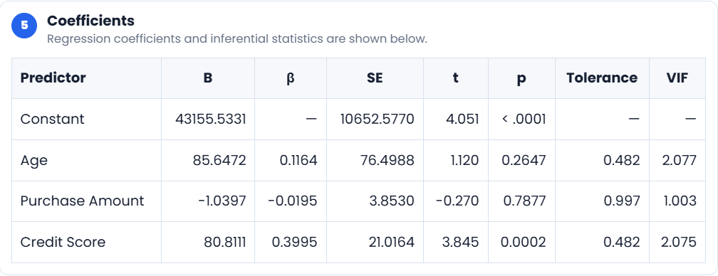

The coefficients table shows that Credit Score is the only statistically significant predictor after adjusting for the other variables (\(B=80.81,\ \beta=.400,\ t=3.845,\ p=.0002\)). Neither Age (\(p=.2647\)) nor Purchase Amount (\(p=.7877\)) makes a statistically significant unique contribution to the fitted model.

The tolerance and VIF statistics indicate that multicollinearity is not a concern, supporting stable estimation of the regression coefficients.

8. Four Layers of Interpretation

Numerical Result. The overall multiple regression model was statistically significant, \(F(3,146)=15.398,\ p<.0001\). The model explained approximately 24.0% of the observed variation in Annual Income (\(R=.490,\ R^2=.240,\ \text{Adjusted }R^2=.225\)). Among the predictors, only Credit Score was statistically significant (\(B=80.81,\ \beta=.400,\ p=.0002\)).

Statistical Interpretation. The null hypothesis that all regression coefficients equal zero is rejected. Collectively, Age, Credit Score, and Purchase Amount significantly predict Annual Income. After controlling for the remaining predictors, Credit Score makes a statistically significant positive contribution, whereas Age and Purchase Amount do not contribute significantly.

Practical Interpretation. Customers with higher Credit Scores tend to have higher predicted Annual Income after accounting for Age and Purchase Amount. Although Age and Purchase Amount may individually relate to Annual Income, they do not explain additional unique variation once Credit Score is included in this model. The diagnostic plots also suggest that one unusual observation should be investigated before drawing strong substantive conclusions.

📝APA Result: A multiple linear regression significantly predicted Annual Income, F(3, 146) = 15.398, p < .001, R² = .240, adjusted R² = .225. Credit Score was a significant positive predictor of Annual Income, \(B=80.81\), \(SE=21.02\), \(\beta=.400\), t(146)=3.845, p=.0002. Age, \(B=85.65\), p=.2647, and Purchase Amount, \(B=-1.04\), p=.7877, did not make statistically significant unique contributions after controlling for the remaining predictors.

9. Key Learning Point

Multiple regression distinguishes between the overall explanatory power of the model and the unique contribution of each predictor. A model may be statistically significant even though only one predictor contributes significantly after the others are controlled. Consequently, the overall F-test, coefficient tests, model fit statistics, and regression diagnostics should always be interpreted together.

Worked Example 7.4: Multiple Regression with Continuous and Binary Predictors

This example demonstrates a multiple regression model containing both continuous and binary predictors. The objective is to determine whether Income, Gender, and Card Loyalty jointly predict Purchase Amount, while illustrating how binary categorical variables are incorporated into regression through dummy coding.

Unlike the previous example, the outcome variable is Purchase Amount. The binary predictors estimate adjusted differences between groups after controlling for the continuous predictor.

1. Research Question

Do Income, Gender, and Card Loyalty significantly predict Purchase Amount, and do the binary predictors represent statistically significant adjusted differences in Purchase Amount after Income has been controlled?

2. Variables

The dependent variable is Purchase Amount.

The predictors are:

• Income — continuous;
• Gender — binary categorical (Male vs Female); and
• Card Loyalty — binary categorical (VIP vs Regular).

Binary categorical predictors are represented using dummy variables. For illustration:

\[ D_1= \begin{cases} 0,&\text{Female}\\ 1,&\text{Male} \end{cases} \] \[ D_2= \begin{cases} 0,&\text{Regular}\\ 1,&\text{VIP} \end{cases} \]

Female and Regular therefore serve as the reference categories. The regression model becomes:

\[ \widehat{\text{Purchase Amount}} = b_0 + b_1(\text{Income}) + b_2D_1 + b_3D_2 \]

The dummy-variable coefficients estimate the adjusted differences between the coded group and the corresponding reference category.

3. Hypotheses

The overall regression model evaluates:

\[ H_0: \beta_{\text{Income}} = \beta_{\text{Gender}} = \beta_{\text{Card Loyalty}} = 0 \] \[ H_1: \text{At least one regression coefficient is non-zero} \]

Each predictor is also evaluated individually. For example:

\[ H_0:\beta_{\text{Gender}}=0 \] \[ H_1:\beta_{\text{Gender}}\neq0 \]

Equivalent hypotheses are tested for Income and Card Loyalty.

The significance level is:

\[ \alpha=.05 \]

4. Assumptions and Testing

The assumptions of multiple linear regression apply to the residuals of the fitted model. Binary predictors themselves are not required to follow a normal distribution.

Linearity: The relationship between Income and the conditional mean of Purchase Amount should be approximately linear. The residual-versus-fitted plot shows no pronounced systematic curvature, although one extremely unusual observation is evident.

Independence: The Durbin–Watson statistic is:

\[ DW=2.000 \]

A value essentially equal to 2 indicates little evidence of first-order residual autocorrelation.

Homoscedasticity: Most residuals are centred around zero across the fitted values. However, the extreme positive residual suggests that one observation may have substantial influence on the fitted model.

Residual normality: The Shapiro–Wilk test reports:

\[ W=.298,\quad p<.001 \]

Residual normality is therefore not supported. The Q–Q plot shows a pronounced upper-tail departure associated with the unusually large residual, and the residual histogram similarly reflects this extreme observation.

Multicollinearity: The tolerance values (0.951–0.978) are high and the VIF values (1.023–1.052) are close to 1, indicating no evidence of problematic multicollinearity.

Overall, the regression assumptions appear reasonably satisfied except for the substantial departure from residual normality caused primarily by the influential observation.

💡Key Idea: Regression coefficients for binary predictors estimate adjusted differences between groups. Their interpretation always depends on the chosen reference category rather than on the categorical variable in general.

5. Formula

The multiple regression model is:

\[ \hat{Y} = b_0+b_1X+b_2D_1+b_3D_2 \]

For this analysis:

\[ \widehat{\text{Purchase Amount}} = b_0 + b_1(\text{Income}) + b_2(\text{Gender}) + b_3(\text{Card Loyalty}) \]

The overall model is evaluated using:

\[ F = \frac{MS_{\text{Regression}}} {MS_{\text{Error}}} \]

Each coefficient is evaluated using:

\[ t = \frac{B}{SE(B)} \]

Using the estimated coefficients, the fitted regression equation is:

\[ \widehat{\text{Purchase Amount}} = 935.263 - 0.0015(\text{Income}) - 109.946(\text{Male}) + 133.950(\text{VIP}) \]

6. Manual Calculation

Suppose a VIP customer is male and has an annual income of 90,000. The fitted value is obtained by substituting these values into the regression equation:

\[ \hat{Y} = 935.263 - 0.0015(90\,000) - 109.946(1) + 133.950(1) \]

The residual is then calculated as:

\[ e_i = Y_i-\hat{Y}_i \]

The Explorer automatically estimates the regression coefficients and calculates fitted values, residuals, standard errors, and significance tests.

7. LearnerBox Statistical Explorer

In the Regression tab, select Multiple Linear Regression. Choose Purchase Amount as the dependent variable and select Income, Gender, and Card Loyalty as predictors.

The Explorer reports:

\[ R=.262 \] \[ R^2=.069 \] \[ \text{Adjusted }R^2=.050 \]

The residual standard error is approximately:

\[ 320.115 \]

The overall regression model is statistically significant:

\[ F(3,146)=3.591,\quad p=.0152 \]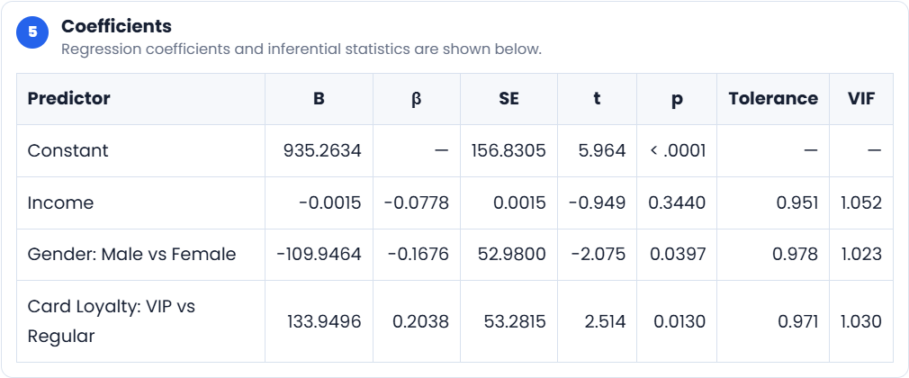

Figure 7.4 presents the adjusted regression coefficients. Income is not statistically significant after controlling for the binary predictors:

\[ B=-0.0015,\quad t=-0.949,\quad p=.344 \]

The Gender coefficient is statistically significant:

\[ B=-109.946,\quad t=-2.075,\quad p=.0397 \]

Because Male is compared with the Female reference category, the negative coefficient indicates that males are predicted to spend approximately 110 units less than females after controlling for Income and Card Loyalty.

Card Loyalty is also statistically significant:

\[ B=133.950,\quad t=2.514,\quad p=.0130 \]

VIP customers are predicted to spend approximately 134 units more than Regular customers after controlling for Income and Gender.

The tolerance and VIF values confirm that multicollinearity is not a concern in this model.

8. Four Layers of Interpretation

Numerical Result

The fitted model is statistically significant with:

\[ F(3,146)=3.591,\quad p=.0152 \]

The model has \(R=.262\), \(R^2=.069\), and adjusted \(R^2=.050\). Approximately 6.9% of the observed variation in Purchase Amount is explained by the predictors.

Statistical Interpretation

The null hypothesis that all regression coefficients equal zero is rejected. However, the significant overall model is driven primarily by the binary predictors. Income does not make a statistically significant unique contribution after Gender and Card Loyalty have been controlled.

Gender (Male vs Female) and Card Loyalty (VIP vs Regular) both make statistically significant adjusted contributions to the model.

Residual normality is not supported by the Shapiro–Wilk test, \(W=.298,\ p<.001\). The extreme positive residual visible in the diagnostic plots should therefore be considered when evaluating the model.

Practical Interpretation

Although the regression model is statistically significant, it explains only a modest proportion of the variability in Purchase Amount. After adjustment, customer group characteristics appear more informative than Income in explaining purchasing behaviour.

Male customers are predicted to spend slightly less than comparable female customers, whereas VIP customers are predicted to spend substantially more than Regular customers. The remaining unexplained variation suggests that many additional customer characteristics influence Purchase Amount.

The regression model describes statistical associations and should not be interpreted as establishing causal relationships.

📝APA Result: A multiple linear regression was conducted to examine whether Income, Gender, and Card Loyalty predicted Purchase Amount. The regression model was statistically significant, F(3, 146) = 3.59, p = .015, \(R^2=.069\), adjusted \(R^2=.050\). Income was not a significant predictor, \(B=-0.0015\), t(146) = -0.95, p = .344. Gender (Male vs Female) was a significant negative predictor, \(B=-109.95\), \(\beta=-.168\), t(146) = -2.08, p = .040, while Card Loyalty (VIP vs Regular) was a significant positive predictor, \(B=133.95\), \(\beta=.204\), t(146) = 2.51, p = .013. Residual diagnostics indicated a substantial departure from normality associated with an influential observation.

9. Key Learning Point

Multiple regression naturally accommodates both continuous and categorical predictors through dummy coding. Continuous predictors estimate linear slopes, whereas binary predictors estimate adjusted differences between groups.

This example illustrates that an overall regression model may be statistically significant even when some individual predictors are not. Interpretation should therefore consider the overall model fit, the individual coefficients, and the diagnostic assessment together.

Practice Exercise 1

A multiple regression model predicts Employee Performance from Years of Experience, Training Hours, and Job Satisfaction. The model is statistically significant, \(F(3,146)=18.40\), \(p<.001\), with \(R^2=.274\) and adjusted \(R^2=.259\). Training Hours has \(p=.018\), Job Satisfaction has \(p<.001\), and Years of Experience has \(p=.214\).

Which predictors make statistically significant unique contributions to the model, and why should Years of Experience not be described as a significant predictor?

Practice Exercise 2

A researcher predicts Customer Spending using Age, Annual Income, and Credit Score. For Annual Income:

Explain the difference between the interpretations of \(B\) and \(\beta\).

Practice Exercise 3

A regression model predicts Examination Score from Study Hours and Teaching Method. Teaching Method is coded:

The coefficient for Teaching Method is:

Interpret the coefficient and explain how this result connects regression with ANOVA.

Binary Logistic Regression

Binary logistic regression is used when the dependent variable has two possible outcomes, such as purchase versus no purchase, default versus no default, or disease present versus disease absent. The outcome is commonly coded as:

The predictors may be continuous, binary, or represented through dummy variables. Logistic regression estimates how the predictors are associated with the probability that the outcome equals 1.

Why Linear Regression Is Unsuitable for Binary Outcomes

Ordinary linear regression is not appropriate for a binary dependent variable. A linear model can produce fitted values below 0 or above 1, even though probabilities must remain within:

The relationship between a predictor and event probability is also generally non-linear. A constant one-unit increase in a predictor does not produce the same absolute change in probability across the entire predictor range. Changes near a probability of .50 can be larger than changes near probabilities close to 0 or 1.

Binary outcomes also violate the constant-variance and normally distributed error structure assumed by ordinary least squares regression. For a Bernoulli outcome:

and:

The conditional variance therefore changes with the predicted probability. Logistic regression addresses these features by modelling a transformed version of probability rather than modelling the binary outcome directly with a straight line.

Probability and Odds

Let \(p\) represent the probability that the event occurs:

The probability that the event does not occur is:

The odds of the event are:

If \(p=.75\), then:

The event has odds of 3 to 1, meaning that the event is expected to occur three times for every one non-event under the specified probability.

If the odds are known, probability can be recovered using:

For odds of 3:

Odds range from 0 to positive infinity. Odds below 1 indicate that the event is less likely than the non-event, odds of 1 correspond to \(p=.50\), and odds above 1 indicate that the event is more likely than the non-event.

Log Odds and the Logit

Logistic regression models the natural logarithm of the odds, called the logit:

The binary logistic regression model is:

The right side of the equation is the linear predictor:

Thus:

Unlike probability, log odds are unbounded and may take any real value. This allows a linear combination of predictors to be modelled without generating invalid probabilities.

The Logistic Function

The logit is transformed back into probability through the logistic function:

Substituting the linear predictor:

The logistic function produces an S-shaped curve. Large negative values of the linear predictor generate probabilities near 0, values near 0 generate probabilities near .50, and large positive values generate probabilities near 1.

The fitted probability is therefore:

This fitted probability can be interpreted directly or converted into a predicted class using a classification threshold, which will be examined in Part 10.

Logistic Regression Coefficients

A logistic regression coefficient \(B_j\) represents the expected change in the log odds of the event for a one-unit increase in predictor \(X_j\), holding the other predictors constant:

If:

then a one-unit increase in \(X_j\) increases the predicted log odds by .40, holding the other predictors constant. Although mathematically correct, log-odds changes are not usually the most intuitive form of interpretation. Coefficients are therefore commonly exponentiated to produce odds ratios.

Odds Ratios

The odds ratio for predictor \(X_j\) is:

An odds ratio describes the multiplicative change in the odds associated with a one-unit increase in the predictor, holding the other predictors constant.

If:

then:

A one-unit increase in the predictor is associated with approximately 1.49 times the odds of the event, equivalent to an approximate 49% increase in odds:

If:

then:

The odds are multiplied by .67, corresponding to an approximate 33% decrease:

An odds ratio of 1 indicates no change in odds. Values above 1 indicate increased odds, whereas values below 1 indicate decreased odds.

Binary Predictors and Reference Categories

A binary predictor is interpreted relative to its reference category. Suppose Loyalty Tier is coded:

The coefficient for \(D\) compares VIP customers with Regular customers, holding the remaining predictors constant. If:

VIP customers have approximately 2.20 times the odds of the event compared with Regular customers at equal values of the other predictors.

Changing the reference category reverses the comparison. The reciprocal odds ratio is:

Thus, Regular customers have approximately .455 times the odds of the event compared with VIP customers.

Wald Tests

Each logistic regression coefficient is commonly evaluated using a Wald test. For predictor \(X_j\):

The Wald statistic is based on the coefficient relative to its standard error:

Some software reports the squared form:

which is evaluated using a chi-square distribution with one degree of freedom.

A statistically significant Wald test indicates that the predictor makes a significant adjusted contribution to the log odds of the event. As in multiple linear regression, each coefficient is interpreted while holding the other predictors constant.

The Wald test may be unstable when coefficients are very large, standard errors are inflated, categories are sparse, or separation is present. In such cases, likelihood-ratio tests or alternative estimation methods may provide more reliable inference.

Maximum Likelihood and Log-Likelihood

Logistic regression coefficients are estimated using maximum likelihood rather than ordinary least squares. Maximum likelihood selects the coefficient values that make the observed pattern of binary outcomes most probable under the fitted model.

For observation \(i\), the Bernoulli likelihood contribution is:

The complete likelihood is:

For computational convenience, software uses the log-likelihood:

A model with a larger log-likelihood, meaning a value closer to zero, fits the observed outcomes better. However, fit must be considered together with model complexity.

Akaike Information Criterion

The Akaike Information Criterion, or AIC, balances model fit against the number of estimated parameters:

where \(\ell\) is the model log-likelihood and \(K\) is the number of estimated parameters.

Lower AIC values indicate a preferable balance of fit and complexity among models fitted to the same outcome and dataset. AIC has no universal interpretation in isolation. A value is meaningful only through comparison with competing models.

Adding predictors may improve log-likelihood but also increases the complexity penalty. A predictor set is therefore favoured only when the improvement in fit is sufficient to justify the additional parameters.

Pseudo-R²

Logistic regression does not have a direct equivalent of the ordinary least squares decomposition used to calculate linear-regression \(R^2\). Several pseudo-\(R^2\) measures have therefore been developed to summarise improvement in fit relative to a baseline model.

McFadden's pseudo-\(R^2\) is:

where \(\ell_{\text{Model}}\) is the log-likelihood of the fitted model and \(\ell_{\text{Null}}\) is the log-likelihood of the intercept-only model.

Larger values indicate greater improvement over the null model. However, McFadden's pseudo-\(R^2\) should not be interpreted using the same scale or language as linear-regression \(R^2\).

Hosmer–Lemeshow Test

The Hosmer–Lemeshow test evaluates the agreement between observed event frequencies and model-predicted probabilities. Cases are commonly grouped according to predicted risk, and observed and expected event counts are compared across those groups.

The hypotheses are:

A non-significant result:

provides insufficient evidence of lack of fit and is generally considered consistent with acceptable calibration. A significant result suggests that observed and predicted event frequencies differ more than expected under the fitted model.

The Hosmer–Lemeshow result should not be treated as a complete measure of model quality. It can be sensitive to sample size and the method used to create probability groups. Calibration plots, discrimination statistics, classification metrics, and substantive plausibility should also be considered.

Evaluating a Logistic Regression Model

A binary logistic regression model should be interpreted at several levels. The coefficient table identifies which predictors make statistically significant adjusted contributions and expresses their effects through odds ratios. Log-likelihood and AIC describe relative model fit, while pseudo-\(R^2\) summarises improvement over the intercept-only model. The Hosmer–Lemeshow test provides one assessment of calibration.

These inferential and fit statistics do not directly answer how accurately the model classifies individual cases. Classification requires predicted probabilities to be converted into predicted outcomes using a threshold. The resulting performance depends on the confusion matrix, sensitivity, specificity, precision, F1-score, and the trade-offs represented by the ROC curve.

The next section develops this predictive perspective by examining classification thresholds and performance measures for binary outcomes.

Classification Performance

A binary logistic regression model produces a predicted probability for each observation:

Statistical inference evaluates whether the predictors contribute to the model and whether the fitted relationships are supported by the data. Classification performance addresses a different question: how effectively can the predicted probabilities be converted into correct outcome classifications? A model may contain statistically significant predictors yet classify cases poorly, while a model with useful predictive performance may include predictors whose individual inferential interpretation is less important. Model inference and predictive performance should therefore be evaluated separately.

Classification Thresholds

Logistic regression produces probabilities rather than classes. To convert a predicted probability into a predicted binary outcome, a classification threshold, denoted by \(c\), is selected:

A commonly used default is:

At this threshold, observations with predicted probabilities of at least .50 are classified as events, while observations below .50 are classified as non-events. However, .50 is a decision convention rather than a universal statistical requirement. The preferred threshold depends on the relative consequences of false-positive and false-negative decisions, the prevalence of the event, and the intended use of the model.

Lowering the threshold classifies more observations as positive. This generally increases sensitivity but also produces more false positives. Raising the threshold classifies fewer observations as positive, usually increasing specificity while increasing the number of false negatives. Threshold selection therefore involves a trade-off rather than a single universally optimal value.

The Confusion Matrix

A confusion matrix compares the observed outcomes with the model's predicted classes. For a binary outcome:

A true positive occurs when the event is observed and the model predicts the event. A true negative occurs when the non-event is observed and the model predicts the non-event. A false positive occurs when the model predicts the event even though the event did not occur. A false negative occurs when the model predicts the non-event even though the event occurred.

The confusion matrix is the foundation for most threshold-dependent classification measures. Different metrics emphasise different combinations of its four cells.

Accuracy

Accuracy is the proportion of all observations classified correctly:

Accuracy is intuitive, but it can be misleading when the outcome classes are imbalanced. If 95% of observations belong to the non-event class, a model that predicts every case as a non-event achieves 95% accuracy while completely failing to identify events.

Accuracy should therefore be interpreted together with class prevalence, sensitivity, specificity, precision, and the confusion matrix.

Sensitivity

Sensitivity, also called recall or the true-positive rate, measures the proportion of observed events correctly identified:

The denominator contains all actual positive cases. High sensitivity indicates that the model misses relatively few events.

Sensitivity is especially important when false negatives are costly. Examples include failing to identify a patient with a serious condition, failing to detect fraud, or failing to identify a customer at high risk of leaving.

Specificity

Specificity, or the true-negative rate, measures the proportion of observed non-events correctly identified:

The denominator contains all actual negative cases. High specificity indicates that the model produces relatively few false-positive classifications.

Specificity becomes particularly important when acting on a false alarm is expensive, disruptive, or harmful. For example, incorrectly flagging legitimate transactions as fraudulent may inconvenience customers and increase investigation costs.

Sensitivity and specificity usually trade off as the classification threshold changes. Lower thresholds tend to increase sensitivity and reduce specificity, while higher thresholds tend to increase specificity and reduce sensitivity.

Precision

Precision, also called the positive predictive value, measures the proportion of predicted positive cases that are actually positive:

Sensitivity asks:

Of all actual events, how many did the model identify?

Precision asks:

Of all cases classified as events, how many were truly events?

Precision is particularly relevant when the cost of investigating or acting on positive predictions is high. A model with low precision generates many false alarms, even if its sensitivity is high.

F1-Score

The F1-score combines precision and recall using their harmonic mean:

The harmonic mean penalises models that perform poorly on either precision or recall. A high F1-score therefore requires both measures to be reasonably strong.

The F1-score is useful when the positive class is important and the analyst wants a single measure balancing false positives and false negatives. However, it does not include true negatives directly and should not replace examination of sensitivity, specificity, and the complete confusion matrix.

Calculating Classification Metrics

Suppose a model produces the following confusion matrix:

The total number of observations is:

Accuracy is:

The model correctly classifies 71% of observations.

Sensitivity is:

The model identifies 80% of the observed positive cases.

Specificity is:

The model correctly identifies 57.5% of the observed negative cases.

Precision is:

Approximately 73.8% of cases classified as positive are actually positive.

The F1-score is:

The example shows why accuracy alone is incomplete. Although overall accuracy is 71%, the model performs better at identifying positive cases than negative cases. Its sensitivity is considerably higher than its specificity.

The ROC Curve

The receiver operating characteristic curve, or ROC curve, evaluates binary classification performance across all possible classification thresholds. For each threshold, it plots:

against:

The horizontal axis therefore represents:

and the vertical axis represents:

Each point on the ROC curve corresponds to a different classification threshold. Lowering the threshold generally moves the operating point towards higher sensitivity and a higher false-positive rate. Raising the threshold generally lowers both rates.

A model with no discriminatory ability follows approximately the diagonal line from \((0,0)\) to \((1,1)\). A model with stronger discrimination bends towards the upper-left corner, where sensitivity is high and the false-positive rate is low.

Area Under the ROC Curve

The area under the ROC curve, or AUC, summarises the model's ability to discriminate between positive and negative cases across thresholds.

Conceptually, AUC can be interpreted as the probability that the model assigns a higher predicted probability to a randomly selected positive case than to a randomly selected negative case.

AUC values range from 0 to 1:

• \(AUC=.50\) indicates no discrimination beyond chance;
• values above .50 indicate increasing discriminatory ability;
• \(AUC=1.00\) indicates perfect discrimination; and
• values below .50 suggest reversed prediction or incorrect outcome coding.

Broad descriptive guidelines sometimes classify AUC values of approximately .70, .80, and .90 as acceptable, good, and excellent discrimination. These conventions should be interpreted in relation to the application, consequences of errors, sample characteristics, and comparison with alternative models.

AUC is threshold-independent, but it does not determine which threshold should be used operationally. Two models with similar AUC values may produce different sensitivity and specificity at a particular decision threshold. AUC also does not directly evaluate calibration—that is, whether predicted probabilities agree with observed event frequencies.

Inference Versus Prediction

A complete logistic regression analysis distinguishes at least three analytical questions:

1. Do the predictors contribute statistically?

Coefficient estimates, Wald tests, confidence intervals, and odds ratios address predictor-level inference.

2. Does the model fit the observed data adequately?

Log-likelihood, AIC, pseudo-\(R^2\), and calibration diagnostics address model fit.

3. How effectively does the model classify cases?

The confusion matrix, accuracy, sensitivity, specificity, precision, F1-score, ROC curve, and AUC address predictive classification performance.

These results may not point in the same direction. A predictor may have a statistically significant odds ratio but produce only a small improvement in classification. A model may achieve reasonable accuracy because the dominant class is easy to predict, yet perform poorly on the minority class. Conversely, a model may discriminate cases effectively while its predicted probabilities require recalibration.

Classification performance should ideally be assessed on data not used to estimate the model. Metrics calculated from the training sample may overstate performance because the model has already been fitted to those observations. Holdout validation or cross-validation provides a more realistic estimate of how the model may perform on new data.

The next worked example applies these ideas to a logistic regression model predicting Repeat Purchase. It interprets the coefficient table, converts coefficients into odds ratios, evaluates model fit, and calculates classification metrics from the confusion matrix.

Worked Example 7.5: Predicting Employment Status with Binary Logistic Regression

Worked Example 7.5

This example uses binary logistic regression to predict whether an individual is employed or unemployed (Employment Status). The model combines continuous and binary predictors, estimates their adjusted effects using log-odds coefficients and odds ratios, and evaluates both model fit and classification performance.

Unlike multiple linear regression, binary logistic regression models the probability of belonging to one of two outcome categories. The fitted model therefore estimates how Age, Income, Savings Balance, and Gender influence the probability that an individual is employed.

1. Research Question

Do Age, Income, Savings Balance, and Gender significantly predict Employment Status, and how accurately can the fitted logistic regression model classify individuals as employed or unemployed?

2. Variables

The dependent variable is Employment Status, coded as:

\[ Y= \begin{cases} 0,&\text{Unemployed}\\ 1,&\text{Employed} \end{cases} \]

The predictors are:

• Age — continuous;
• Income — continuous;
• Savings Balance — continuous; and
• Gender — binary categorical.

Gender is represented using dummy coding. In this example the Explorer compares Male with the reference category Female, so the coefficient estimates the adjusted difference in employment odds between males and females while the continuous predictors are held constant.

3. Hypotheses

The overall logistic regression model evaluates:

\[ H_0: \beta_{\text{Age}} = \beta_{\text{Income}} = \beta_{\text{Savings Balance}} = \beta_{\text{Gender}} = 0 \] \[ H_1: \text{At least one regression coefficient is non-zero} \]

Each predictor is also evaluated individually. For example, Age is tested using:

\[ H_0:\beta_{\text{Age}}=0 \] \[ H_1:\beta_{\text{Age}}\neq0 \]

Equivalent coefficient hypotheses are tested for Income, Savings Balance, and Gender.

The significance level is:

\[ \alpha=.05 \]

4. Assumptions and Model Conditions

Binary logistic regression is appropriate because the outcome variable contains two categories and each observation contributes independently to the analysis.

Unlike ordinary least squares regression, logistic regression models the relationship between the predictors and the log odds of Employment Status rather than the observed outcome itself. Consequently, normally distributed residuals and constant residual variance are not required assumptions.

Linearity of the logit: The continuous predictors should have approximately linear relationships with the log odds of Employment Status. The fitted probability plot indicates that the model captures the observed probabilities well across the range of Age.

Independence of observations: Each participant contributes a single independent observation to the analysis.

Multicollinearity: The tolerance values range from approximately 0.733 to 0.946, while the VIF values range from approximately 1.06 to 1.37. These values are well below commonly used thresholds, indicating no evidence of problematic multicollinearity among the predictors.

Model discrimination: The ROC curve lies well above the chance line and the area under the curve is:

\[ \text{AUC}=.987 \]

This indicates outstanding discrimination between employed and unemployed individuals.

Calibration: The calibration plot shows predicted probabilities that generally agree closely with the observed event proportions, particularly at the upper end of the probability scale.

📋Remember: Binary logistic regression does not require normally distributed residuals. Instead, emphasis is placed on appropriate outcome coding, independence of observations, linearity of the logit for continuous predictors, absence of serious multicollinearity, and evaluation of predictive performance through measures such as ROC curves and classification accuracy.

5. Formula

Binary logistic regression models the log odds of the outcome:

\[ \log\left(\frac{p}{1-p}\right) = \beta_0 + \beta_1(\text{Age}) + \beta_2(\text{Income}) + \beta_3(\text{Savings Balance}) + \beta_4(\text{Gender}) \]

where \(p\) is the probability that an individual is employed.

The fitted probability is obtained from:

\[ \hat{p} = \frac{1} { 1+ e^{ - \left[ b_0 + b_1(\text{Age}) + b_2(\text{Income}) + b_3(\text{Savings Balance}) + b_4(\text{Gender}) \right] } } \]

Each coefficient may be transformed into an odds ratio using:

\[ OR=e^B \]

An odds ratio greater than 1 indicates increased odds of employment as the predictor increases (or for the coded category), whereas an odds ratio less than 1 indicates reduced odds of employment after the remaining predictors have been held constant.

6. Manual Calculation

One of the most useful interpretations in binary logistic regression is the conversion of a log-odds coefficient into an odds ratio. For Age, the estimated coefficient is:

\[ B=-0.1013 \]

The corresponding odds ratio is:

\[ OR=e^{-0.1013} \] \[ OR\approx0.904 \]

Holding Income, Savings Balance, and Gender constant, each additional year of age multiplies the odds of being employed by approximately 0.904.

Because this odds ratio is less than 1, increasing Age is associated with a reduction in the odds of employment. Expressed as a percentage:

\[ (1-0.904)\times100 = 9.6\% \]

Each additional year of age is therefore associated with an approximate 9.6% decrease in the odds of employment, after controlling for the remaining predictors.

Savings Balance has an estimated coefficient of:

\[ B=0.0005 \]

The corresponding odds ratio is:

\[ OR=e^{0.0005}\approx1.001 \]

Although the coefficient appears numerically small because Savings Balance is measured in currency units, the positive odds ratio indicates that larger savings balances are associated with higher odds of employment after the remaining predictors have been held constant.

💡Key Idea:

Logistic regression coefficients are interpreted most naturally through their odds ratios. A positive coefficient corresponds to an odds ratio greater than 1, whereas a negative coefficient corresponds to an odds ratio less than 1. The size of the coefficient must always be interpreted relative to the units in which the predictor is measured.

7. LearnerBox Statistical Explorer

In the Regression tab, select Binary Logistic Regression. Choose Employment Status as the dependent variable and select Age, Income, Savings Balance, and Gender as predictors.

The model summary reports:

\[ N=150 \] \[ \text{Log-likelihood}=-12.874 \] \[ AIC=35.748 \] \[ R_{\text{McFadden}}^2=.757 \] \[ R_{\text{Nagelkerke}}^2=.818 \] \[ AUC=.987 \]

The pseudo-\(R^2\) statistics indicate an excellent improvement over the intercept-only model, while the ROC AUC of .987 demonstrates outstanding discrimination between employed and unemployed individuals.

Unlike ordinary least squares regression, pseudo-\(R^2\) measures should not be interpreted as the exact proportion of variance explained. Instead, they quantify improvement in model fit relative to a model containing only the intercept.

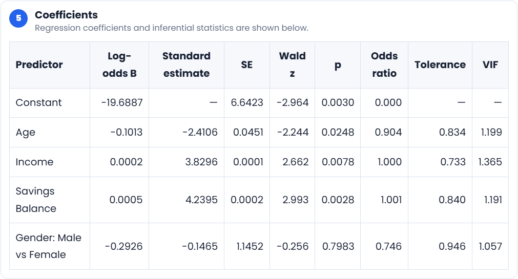
Figure 7.5 reports the log-odds coefficients, standardised estimates, standard errors, Wald statistics, p-values, odds ratios, tolerance values, and VIF statistics for each predictor.

The log-odds B column reports the estimated regression coefficient for each predictor on the logit scale. Each coefficient represents the expected change in the log odds of being employed associated with a one-unit increase in a continuous predictor, or the change from the reference category to the coded category for a binary predictor, while all other predictors are held constant. Positive coefficients increase the log odds (and therefore the probability) of employment, whereas negative coefficients decrease the log odds. Because log odds are difficult to interpret directly, the corresponding odds ratio, obtained by exponentiating the coefficient, is usually the preferred measure for practical interpretation.

The SE (standard error) column measures the sampling variability of each estimated coefficient. Smaller standard errors indicate that the coefficient has been estimated more precisely, whereas larger standard errors reflect greater uncertainty in the estimate. The standard error is used to calculate the Wald test statistic, which evaluates whether the coefficient differs significantly from zero after accounting for sampling variability. Consequently, both the magnitude of the coefficient and its standard error determine whether a predictor makes a statistically significant unique contribution to the logistic regression model.

Age is a statistically significant predictor of Employment Status (\(p=.0248\)). Its odds ratio of 0.904 indicates that increasing age is associated with lower odds of employment after the remaining predictors have been held constant.

Income is also statistically significant (\(p=.0078\)). Although its coefficient is numerically small because Income is measured in currency units, the positive coefficient indicates that higher income is associated with greater odds of employment.

Savings Balance is likewise statistically significant (\(p=.0028\)), with an odds ratio slightly above 1, indicating increased odds of employment as savings increase.

Gender does not make a statistically significant unique contribution to the model (\(p=.7983\)). After Age, Income, and Savings Balance have been controlled, the data provide insufficient evidence of an adjusted difference in employment status between males and females.

⚠️Common Mistake: Do not judge predictor importance solely from the numerical size of the coefficient. Predictors measured in different units naturally have coefficients of different magnitudes. Statistical significance, odds ratios, and subject-matter interpretation should always be considered together.

Classification Performance

The Explorer applies a classification threshold of:

\[ c=.50 \]

The confusion matrix reports:

\[ TN=14,\quad FP=3,\quad FN=3,\quad TP=130 \]

	Predicted 0	Predicted 1
Actual 0	14	3
Actual 1	3	130

The classification performance statistics are:

\[ \text{Accuracy}=.960 \] \[ \text{Sensitivity}=.977 \] \[ \text{Specificity}=.824 \] \[ \text{Precision}=.977 \] \[ F_1=.977 \]

The model correctly classifies 96.0% of observations. It identifies 97.7% of employed individuals correctly (sensitivity) while correctly identifying 82.4% of unemployed individuals (specificity). Precision and the F1-score are also exceptionally high, indicating highly reliable classification performance.

The ROC curve supports these results. An AUC of .987 indicates excellent discrimination and shows that the fitted model almost perfectly distinguishes employed from unemployed individuals across a wide range of classification thresholds.

8. Four Layers of Interpretation

Numerical Result: The binary logistic regression model produced a log-likelihood of \(-12.874\), AIC of 35.748, McFadden pseudo-\(R^2=.757\), Nagelkerke pseudo-\(R^2=.818\), and ROC AUC of .987. At the .50 threshold, accuracy was .960, sensitivity was .977, specificity was .824, precision was .977, and the F1-score was .977.

Statistical Interpretation: Age, Income, and Savings Balance make statistically significant adjusted contributions to the probability of employment. Gender does not make a statistically significant unique contribution after the remaining predictors have been controlled. The predictor set therefore provides strong evidence for explaining Employment Status.

Practical Interpretation: The model demonstrates outstanding predictive performance. Increasing Income and Savings Balance are associated with higher odds of employment, whereas increasing Age is associated with lower odds of employment after adjustment for the other predictors. Gender contributes little additional predictive information in this model.

📝APA Result: A binary logistic regression model significantly predicted Employment Status using Age, Income, Savings Balance, and Gender. The model demonstrated excellent fit (McFadden pseudo-R² = .757; Nagelkerke pseudo-R² = .818) and outstanding discrimination (ROC AUC = .987). Age (OR = 0.904, p = .025), Income (p = .008), and Savings Balance (p = .003) were statistically significant predictors of Employment Status, whereas Gender did not make a statistically significant unique contribution (p = .798). Using a .50 classification threshold, the model achieved 96.0% accuracy, 97.7% sensitivity, 82.4% specificity, 97.7% precision, and an F1-score of .977.

9. Key Learning Point

Binary logistic regression should be interpreted at several complementary levels. Coefficient estimates and Wald tests evaluate the adjusted contribution of individual predictors, odds ratios quantify multiplicative changes in the odds of the outcome, likelihood-based statistics evaluate overall model fit, and classification measures assess predictive performance.

This example demonstrates that a logistic regression model can provide both strong statistical evidence and excellent predictive performance. Nevertheless, individual predictors should always be interpreted alongside model diagnostics and classification metrics to obtain a complete understanding of the fitted model.

Practice Exercise 1

A logistic regression coefficient for Customer Tenure is:

Calculate the odds ratio and interpret the result.

Practice Exercise 2

A binary predictor is coded:

Its logistic regression coefficient and odds ratio are:

Interpret the result.

Practice Exercise 3

A classification model produces:

Calculate accuracy, sensitivity, specificity, and precision. Briefly describe the model's performance.

Choosing and Evaluating Regression Models

The appropriate analytical method depends on the outcome variable, the number of predictors, and the purpose of the analysis. Correlation and regression are related, but they answer different questions. Linear and logistic regression also belong to the same modelling framework, but they represent different types of outcomes and use different estimation and interpretation methods.

Correlation versus Regression

Pearson's correlation describes the direction and strength of the linear association between two quantitative variables:

Correlation is symmetric:

Interchanging the variables does not change the correlation coefficient. Neither variable is formally designated as the predictor or outcome.

Regression assigns distinct roles to the variables. One variable is treated as the outcome, and one or more variables are used as predictors. Regression produces a fitted equation, estimates expected changes in the outcome, generates predicted values, and separates explained from residual variation.

Use correlation when the objective is to quantify a bivariate linear association. Use regression when the objective is to model an outcome, estimate predictor coefficients, adjust for additional variables, or generate predictions.

Simple versus Multiple Linear Regression

Use simple linear regression when the outcome is continuous and the model contains one predictor:

The model estimates one slope and describes the expected change in the outcome for a one-unit increase in the predictor. In simple regression with an intercept:

Use multiple linear regression when the outcome is continuous and the model contains two or more predictors:

Multiple regression estimates the adjusted contribution of each predictor while holding the remaining predictors constant. It also allows continuous and dummy-coded categorical predictors to be included within the same model.

The choice should be driven by the research question and substantive model rather than by a desire to maximise \(R^2\). Adding predictors increases model complexity and may introduce multicollinearity, unstable coefficients, or overfitting. Model comparison should therefore consider adjusted \(R^2\), diagnostic evidence, theoretical relevance, and predictive validation.

Linear versus Logistic Regression

The type of dependent variable determines whether linear or logistic regression is appropriate. Use linear regression when the outcome is continuous and its conditional mean can be represented through a linear predictor:

Use binary logistic regression when the outcome has two categories:

Logistic regression models the log odds of the event:

Linear-regression coefficients describe expected changes in the outcome's original units. Logistic-regression coefficients describe changes in log odds and are commonly exponentiated to obtain odds ratios:

The two model types also use different evaluation measures. Linear regression uses statistics such as \(R^2\), adjusted \(R^2\), residual standard error, F-tests, coefficient t-tests, and residual diagnostics. Logistic regression uses likelihood-based fit measures, AIC, pseudo-\(R^2\), Wald tests, odds ratios, calibration diagnostics, and classification-performance measures.

Explanatory versus Predictive Models

An explanatory model is primarily concerned with estimating and interpreting relationships. Predictor selection is guided by theory, prior evidence, confounding control, and the inferential question. Coefficients, standard errors, confidence intervals, p-values, assumptions, and substantive interpretation receive particular emphasis.

A predictive model is primarily evaluated by its performance on observations not used to estimate the model. The objective is to generate accurate predictions or classifications. Holdout samples, cross-validation, prediction error, calibration, discrimination, and threshold-dependent performance become central.

The two objectives overlap, but they are not interchangeable. A statistically significant coefficient may produce little improvement in prediction. A model with strong in-sample fit may perform poorly on new data. Conversely, a model may predict effectively while individual coefficients remain difficult to interpret because of multicollinearity, non-linear transformations, or complex feature construction.

Decision Process for Model Selection

A practical model-selection sequence begins with the dependent variable and then considers the number and role of the predictors.

Step 1: Is the objective only to describe the association between two quantitative variables?

Use Pearson's correlation when the relationship is approximately linear and its assumptions are reasonable.

Step 2: Is there a continuous dependent variable?

Use simple linear regression for one predictor and multiple linear regression for two or more predictors.

Step 3: Is the dependent variable binary?

Use binary logistic regression to model the probability of the event.

Step 4: Are categorical predictors included?

Represent categorical predictors through appropriate dummy variables and clearly identify the reference category.

Step 5: Is the objective explanatory, predictive, or both?

For explanatory analysis, prioritise theory, adjusted coefficient interpretation, inferential uncertainty, and diagnostics. For predictive analysis, prioritise validation and performance on data not used for model estimation.

Step 6: Are the model conditions reasonable?

Examine residual structure, functional form, independence, unusual observations, multicollinearity, calibration, and other diagnostics appropriate to the selected model.

Step 7: Does the model provide practically useful performance?

Interpret statistical significance together with effect magnitude, explained variation, prediction error, discrimination, calibration, and the practical consequences of incorrect decisions.

Module Summary

This module extended statistical inference from comparisons among means to models of relationships and prediction. Correlation provided a concise measure of bivariate linear association, while regression assigned distinct roles to predictors and outcomes and represented those relationships through fitted equations.

Pearson's correlation quantified the direction and strength of the linear association between Age and Annual Income. The corresponding simple linear regression expressed the same relationship as a fitted prediction equation and showed that:

when the model contains one predictor and an intercept.

Simple linear regression introduced the intercept, slope, fitted values, residuals, and least-squares estimation. Total outcome variation was partitioned into regression and residual components, continuing the variance-partitioning logic developed in ANOVA. The model F-test evaluated the fitted model as a whole, while the coefficient t-test evaluated the slope.

Regression diagnostics shifted the analytical process from simply fitting a model to critically evaluating it. Residual-versus-fitted plots were used to assess linearity and homoscedasticity, Q–Q plots and Shapiro–Wilk tests assessed residual normality, and the Durbin–Watson statistic examined first-order autocorrelation. Outliers, leverage, influence, and Cook's distance distinguished different ways in which individual observations may affect a regression model.

Multiple linear regression incorporated several predictors simultaneously. Each coefficient represented an adjusted association while the other predictors were held constant. Unstandardised coefficients \(B\) retained the original measurement units, whereas standardised coefficients \(\beta\) expressed adjusted relationships in standard deviation units. The model F-test evaluated the predictors jointly, while coefficient t-tests evaluated their individual contributions.

The distinction between \(R^2\) and adjusted \(R^2\) became important as model complexity increased. Multicollinearity was assessed using tolerance and VIF because substantial overlap among predictors can inflate standard errors and destabilise individual coefficients even when overall model fit remains adequate.

Dummy coding incorporated categorical predictors into the regression framework. A binary-predictor coefficient represented the adjusted difference between the category coded 1 and the reference category coded 0. This established the connection between ANOVA and regression: both can represent group differences within the general linear modelling framework.

Binary logistic regression extended modelling to outcomes coded 0 and 1. The model represented predictors as a linear function of log odds and transformed the resulting values into predicted probabilities using the logistic function. Exponentiating a coefficient produced an odds ratio, which described the multiplicative change in event odds associated with a predictor while the remaining predictors were held constant.

Likelihood, AIC, pseudo-\(R^2\), and the Hosmer–Lemeshow test evaluated different aspects of logistic model fit. These measures were distinguished from classification performance. Predicted probabilities were converted into classes using a threshold, and the resulting confusion matrix provided accuracy, sensitivity, specificity, precision, and F1-score. ROC curves and AUC assessed discrimination across classification thresholds.

Across the five worked examples, the module developed a complete modelling workflow:

Visualise the relationship → specify the outcome and predictors → fit the model → assess overall fit → interpret coefficients → diagnose assumptions and influential observations → evaluate predictive performance → report the result in context.

Key Takeaways

• Correlation quantifies bivariate linear association, whereas regression specifies an outcome and one or more predictors.
• Pearson's \(r\) describes direction and strength but does not establish causation.
• Simple linear regression models a continuous outcome using one predictor.
• The intercept is the predicted outcome when the predictor equals zero, while the slope is the expected outcome change associated with a one-unit predictor increase.
• Least squares estimates the line that minimises the sum of squared residuals.
• Residuals are the differences between observed and fitted outcome values.
• In simple regression with one predictor and an intercept, \(R^2=r^2\).
• \(R^2\) describes in-sample explained variation, while adjusted \(R^2\) penalises unnecessary model complexity.
• The model F-test evaluates the predictor set as a whole, while coefficient tests evaluate individual predictors.
• Regression assumptions concern the functional form and residual structure of the fitted model.
• Outliers have unusual residuals, high-leverage observations have unusual predictor values, and influential observations materially affect the fitted model.
• Cook's distance combines residual magnitude and leverage to assess influence.
• Multiple regression coefficients are interpreted while holding the other predictors constant.
• Unstandardised coefficients \(B\) retain original measurement units, while standardised coefficients \(\beta\) use standard deviation units.
• A statistically significant model may contain non-significant individual predictors.
• Tolerance and VIF assess linear overlap among predictors and the resulting inflation of coefficient uncertainty.
• Dummy coding represents categorical predictors through comparisons with a reference category.
• A binary dummy coefficient in linear regression represents an adjusted mean difference.
• Binary logistic regression models event log odds and converts them into probabilities through the logistic function.
• Exponentiating a logistic coefficient produces an odds ratio.
• An odds ratio describes a multiplicative change in odds, not a direct percentage-point change in probability.
• AIC compares the balance of fit and complexity among models fitted to the same outcome and data.
• Pseudo-\(R^2\) should not be interpreted as ordinary variance explained.
• The Hosmer–Lemeshow test evaluates one aspect of logistic-model calibration but does not prove that the model is correct.
• A classification threshold converts predicted probabilities into predicted classes.
• Accuracy, sensitivity, specificity, precision, and F1-score emphasise different classification objectives.
• ROC curves show the sensitivity–false-positive trade-off across thresholds, while AUC summarises discrimination.
• Calibration and discrimination are distinct properties of a classification model.
• Statistical significance, model fit, practical importance, and predictive performance answer different questions.
• Predictive performance should ideally be evaluated using holdout data or cross-validation.
• The appropriate model is determined by the outcome type, predictor structure, research question, and analytical purpose.