

If you find the content useful and wish to support our platform’s development, you can contribute any amount toward our production costs. Scan the UPI QR code for payment within India. Or use the Ko-fi link to process a secure payment via PayPal.
If you find the content useful and wish to support our platform’s development, you can contribute any amount toward our production costs. Scan the UPI QR code for payment within India. Or use the Ko-fi link to process a secure payment via PayPal.
In Module 5, hypothesis testing focused primarily on comparisons involving one or two means. The one-sample t-test compared a sample mean with a hypothesised population value, while the independent-samples t-test examined whether the means of two independent populations differed. These procedures introduced a general inferential framework in which an observed difference is evaluated relative to the variability expected under the null hypothesis. The magnitude of the test statistic, together with its sampling distribution and the selected significance level, provides the basis for deciding whether the observed result is sufficiently inconsistent with \(H_0\). However, many research designs extend beyond comparisons involving only two groups. A researcher may need to compare Annual Income across several regions, customer spending across multiple loyalty categories, or performance scores across several experimental conditions. Once three or more population means are considered simultaneously, the analytical problem becomes broader than the comparison addressed by a single independent-samples t-test.
One apparent solution is to conduct a separate t-test for every possible pair of groups. Suppose Annual Income is compared across four regions: North, South, East, and West. The researcher could compare North with South, North with East, North with West, South with East, South with West, and East with West. In general, the number of unique pairwise comparisons among \(k\) groups is given by \(\frac{k(k-1)}{2}\). Four groups therefore require six pairwise tests, five groups require ten, and six groups require fifteen. Although each individual t-test remains a valid test of its own pairwise hypothesis, a collection of repeated t-tests does not provide an efficient inferential framework for evaluating the complete set of population means. More importantly, each additional hypothesis test creates another opportunity to reject a true null hypothesis. The difficulty is therefore not merely the increasing number of calculations; repeated testing alters the error properties of the overall analysis.
This problem is understood through the familywise error rate. Recall that when a hypothesis test is conducted at \(\alpha=.05\), the probability of a Type I error is 5% when the null hypothesis is true. This error rate applies to the individual test. If several hypotheses belonging to the same family are tested separately, the probability of making at least one Type I error across the collection of tests becomes greater than the nominal alpha level. Under the simplifying assumption that the tests are independent, the familywise error rate for \(m\) tests can be expressed as:
\[ FWER = 1-(1-\alpha)^m \]For example, consider six pairwise tests conducted at \(\alpha=.05\). The probability of avoiding a Type I error in a single test is \(.95\). The probability of avoiding a Type I error across all six tests is approximately \((.95)^6=.735\). Consequently, the probability of making at least one Type I error is \(1-.735=.265\), or approximately 26.5%. Thus, although every individual comparison uses a 5% significance level, the probability of obtaining at least one false-positive result across the family of six comparisons is substantially larger. This accumulation of Type I error is commonly described as alpha inflation. Multiple-comparison adjustments can be used to control the familywise error rate, but when the original research question concerns the equality of several population means, beginning with a series of separate pairwise tests is generally not the appropriate primary analytical strategy.
Analysis of Variance (ANOVA) was developed to address this broader mean-comparison problem. Instead of testing population means two at a time, ANOVA evaluates the complete set of means within a single omnibus hypothesis test. For \(k\) groups, the null hypothesis states that all population means are equal:
\[ H_0:\mu_1=\mu_2=\cdots=\mu_k \]The alternative hypothesis states that the complete equality specified by \(H_0\) does not hold. In practical terms, at least one population mean differs from at least one other population mean. This distinction is fundamental to the interpretation of ANOVA. A statistically significant omnibus test provides evidence that the population means are not all equal, but it does not establish that every mean differs from every other mean, nor does it identify the particular groups responsible for the significant result. When the omnibus null hypothesis is rejected, appropriate follow-up procedures may be required to determine where the differences occur.
The name Analysis of Variance may initially appear unusual because ANOVA is commonly used to answer questions about differences between means. The logic of the procedure becomes clearer when the sources of variability in the data are considered. Observations within the same group differ from one another, producing within-group variability. At the same time, the group means may differ, producing between-group variability. If the null hypothesis is true and the population means are equal, differences among the observed sample means should primarily reflect sampling fluctuation and the same underlying error variation that produces differences among observations within the groups. If the population means are genuinely different, group membership contributes systematic variation, and the variability among the group means becomes larger relative to the residual variability within the groups.
ANOVA formalises this comparison through the F-ratio. The between-group mean square represents variation associated with differences among the group means, while the within-group mean square represents residual variation among observations belonging to the same groups. The basic F statistic is expressed as:
\[ F = \frac{MS_{\text{Between}}}{MS_{\text{Within}}} \]When the null hypothesis is true, the numerator and denominator provide estimates of the same underlying error variance, apart from sampling fluctuation, and the F-ratio tends to remain relatively close to 1. As systematic differences among the group means increase relative to within-group variation, the numerator becomes larger in relation to the denominator and the F statistic increases. The inferential question is therefore whether the observed ratio of systematic to residual variation is sufficiently large to be unlikely under the null hypothesis.
The motivation for ANOVA therefore extends beyond the practical need to compare three or more means. It introduces a more general statistical perspective in which total variability is partitioned into components associated with identifiable sources. In a one-way ANOVA, a single categorical factor is examined as a source of systematic variation in a continuous dependent variable. In a two-way ANOVA, two factors are incorporated into the same model, allowing the analysis to estimate the main effect of each factor and determine whether the effect of one factor depends on the level of the other. This latter relationship is represented by an interaction effect.
The progression from t-tests to ANOVA is thus an important step towards model-based statistical analysis. The central question is no longer restricted to whether one mean differs from another. Instead, we ask how the observed variability in a dependent variable can be partitioned into systematic components associated with the factors under investigation and residual variation that remains unexplained by the model. This logic forms the foundation of ANOVA and will also reappear in regression and more advanced statistical modelling.
By the end of this module, you should be able to:
ANOVA begins with a fundamental statistical question: why do observations differ from one another? In almost any dataset, values of a continuous variable show variation. Customers differ in their Annual Income, Purchase Amount, and Credit Score; students differ in assessment performance; and patients differ in treatment outcomes. Statistical modelling attempts to determine whether some of this observed variability can be systematically associated with variables included in the model. The remaining variation is treated as residual or unexplained variability.
Consider a study comparing a continuous dependent variable across several groups. If the group means are nearly identical and observations vary considerably within each group, knowing a person's group membership provides little information about the likely value of the dependent variable. Most of the observed variation remains within the groups. In contrast, if the group means are substantially separated and observations within each group are relatively similar, group membership accounts for a meaningful component of the variation in the dependent variable. In this situation, the grouping factor is said to explain part of the variability in the outcome.
The term explained variance does not imply that the statistical model has identified a complete causal explanation for the dependent variable. Rather, it indicates that a component of the observed variability is statistically associated with the factor or factors included in the model. ANOVA therefore separates variation that is systematically associated with the model from variation that remains within the groups and is not accounted for by the grouping factor.
This perspective represents an important development from the t-tests studied in Module 5. A t-test focuses directly on a mean difference and asks whether that difference is large relative to its standard error. ANOVA expresses the same broader inferential logic through variance partitioning. The analysis asks whether variability associated with differences among group means is sufficiently large relative to the variability that remains within the groups.
The total variability in a dependent variable can be partitioned into components representing different sources of variation. In a one-way ANOVA, the primary distinction is between between-group variation and within-group variation. Between-group variation reflects differences among the group means, whereas within-group variation reflects differences among individual observations belonging to the same group.
Suppose Annual Income is compared across four regions. Each region has its own sample mean, and the complete dataset has an overall mean known as the grand mean. If the regional means differ substantially from the grand mean, between-group variation will be relatively large. The grouping variable, Region, is then associated with systematic differences in Annual Income. If the regional means lie close to the grand mean, between-group variation will be relatively small.
Within each region, however, individual incomes also differ from their respective group mean. Some customers earn more than the mean income for their region and others earn less. These individual deviations contribute to within-group variation. Within-group variation is also referred to as error variation or residual variation because it represents variability that is not explained by the grouping factor in the ANOVA model.
The relationship between these components can be written as:
\[ SS_{\text{Total}} = SS_{\text{Between}} + SS_{\text{Within}} \]Here, \(SS\) denotes a sum of squares, a measure of variability based on squared deviations. The total sum of squares measures the overall variability of observations around the grand mean. The between-group sum of squares measures variation associated with differences between the group means and the grand mean. The within-group sum of squares measures variation of individual observations around their respective group means.
Conceptually, the total deviation of an observation from the grand mean can be decomposed into two parts:
\[ x_{ij}-\bar{x}_{..} = (\bar{x}_{i.}-\bar{x}_{..}) + (x_{ij}-\bar{x}_{i.}) \]The term \(x_{ij}\) represents observation \(j\) in group \(i\), \(\bar{x}_{i.}\) represents the mean of group \(i\), and \(\bar{x}_{..}\) represents the grand mean. The first component reflects the position of the group mean relative to the grand mean, while the second reflects the position of the individual observation relative to its own group mean. ANOVA formalises this decomposition across all observations in the dataset.
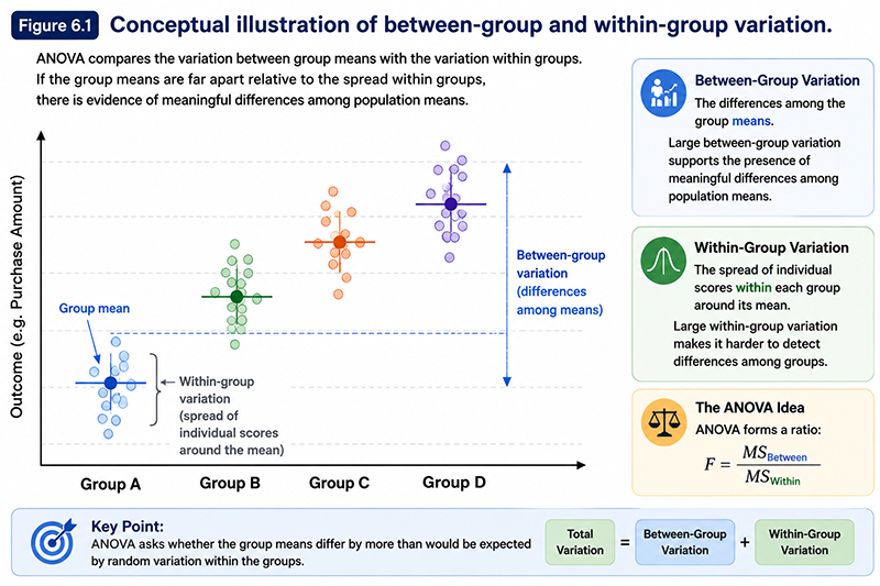
Figure 6.1 illustrates this distinction conceptually. When group means are separated but the observations within each group remain tightly clustered, between-group variation is large relative to within-group variation. When the groups overlap substantially, differences among the group means may be small compared with the variability of observations within the groups.
Sums of squares quantify variability, but they cannot be compared directly without considering their associated degrees of freedom. ANOVA therefore converts each sum of squares into a mean square. A mean square is a variance estimate obtained by dividing a sum of squares by its corresponding degrees of freedom.
For a one-way ANOVA with \(k\) groups and \(N\) total observations, the degrees of freedom are:
\[ df_{\text{Between}} = k-1 \] \[ df_{\text{Within}} = N-k \]The corresponding mean squares are:
\[ MS_{\text{Between}} = \frac{SS_{\text{Between}}}{df_{\text{Between}}} \] \[ MS_{\text{Within}} = \frac{SS_{\text{Within}}}{df_{\text{Within}}} \]These two variance estimates form the basis of the F statistic:
\[ F = \frac{MS_{\text{Between}}}{MS_{\text{Within}}} \]The logic of the F-ratio is central to ANOVA. Under the null hypothesis that all population means are equal, both the between-group and within-group mean squares estimate the same underlying population error variance. Sampling variability may cause the estimates to differ, but neither should be systematically larger than the other. Consequently, an F statistic near 1 is generally consistent with the null hypothesis.
When the population means differ, the between-group mean square contains two sources of variability: random error and systematic variability associated with the grouping factor. The within-group mean square continues to estimate residual error variation. As the systematic component increases, \(MS_{\text{Between}}\) becomes larger relative to \(MS_{\text{Within}}\), producing a larger F statistic.
For example, an F statistic of \(F=1.08\) indicates that the estimated between-group variance is only slightly larger than the estimated within-group variance. An F statistic of \(F=8.50\), in contrast, indicates that the numerator is 8.5 times the denominator. Whether an observed F statistic is statistically significant depends on the F distribution, the numerator and denominator degrees of freedom, and the selected significance level.
Unlike the normal and t distributions examined previously, the F distribution cannot contain negative values because it represents a ratio of variance estimates. Its distribution is typically positively skewed, particularly when the degrees of freedom are small, and the rejection region lies in the right tail. The p-value represents the probability, under the null hypothesis, of obtaining an F statistic at least as large as the observed value.
The statistical decision follows the same hypothesis-testing framework used in Module 5. If \(p<\alpha\), the omnibus null hypothesis is rejected. If \(p\geq\alpha\), the null hypothesis is not rejected. The interpretation, however, concerns the complete set of population means rather than one specific pairwise difference.
The validity of the classical ANOVA F-test depends on assumptions concerning the structure and distribution of the data. These assumptions should be considered as part of the analytical workflow rather than treated as a separate checklist performed after the test. For a standard between-subjects ANOVA, the principal assumptions are independence of observations, normality of residuals, and homogeneity of variance. The dependent variable should also be measured at a continuous level, while the factor variables define categorical groups.
Independence of observations requires that one observation does not systematically determine or influence another observation in the analysis. Independence is primarily a property of the research design and data-collection process; it cannot usually be established through a statistical significance test. Random sampling, random assignment, and appropriate study design help support the assumption. Repeated measurements from the same participant, matched observations, or clustered data violate the independence structure assumed by a standard between-subjects ANOVA and generally require a different analytical model.
The normality assumption applies more precisely to the residuals of the ANOVA model rather than requiring the raw dependent variable to be perfectly normally distributed in every group. Residuals represent the differences between observed values and the values predicted by the model. Their distribution may be examined using graphical procedures such as Q-Q plots and formal tests such as the Shapiro-Wilk test. A non-significant Shapiro-Wilk result provides insufficient evidence to reject the null hypothesis of normality, whereas a significant result suggests a departure from normality. As discussed for t-tests, formal normality tests should be interpreted together with graphical evidence, sample size, and the severity of the departure.
Homogeneity of variance assumes that the population variances are approximately equal across the groups being compared. Levene's test is commonly used to assess this assumption. The null hypothesis of Levene's test states that the group variances are equal. A non-significant result is consistent with homogeneity of variance, while a significant result provides evidence that the variances differ. The importance of a violation depends partly on the degree of variance inequality and whether the group sample sizes are balanced. Classical ANOVA is generally more robust when group sizes are similar, whereas unequal variances combined with substantially unequal sample sizes can distort the F-test.
Assumption testing should therefore inform the choice and interpretation of the statistical model. Minor departures from normality do not automatically invalidate ANOVA, particularly with reasonable sample sizes and balanced groups. However, serious outliers, strongly non-normal residuals, unequal variances, or dependent observations require closer examination. Depending on the nature of the violation, possible responses include data verification, robust procedures, Welch's ANOVA, transformation, or statistical models designed for different dependence structures.
The assumptions establish the conditions under which the F-ratio can be interpreted as a valid comparison of systematic and residual variation. With this conceptual foundation in place, we can now examine how sums of squares are calculated and how the ANOVA table organises the components of variance into a complete inferential model.
A one-way Analysis of Variance (ANOVA) is used to compare the means of a continuous dependent variable across the levels of one categorical independent variable. The categorical variable is commonly referred to as a factor, and its categories are called levels. For example, if Annual Income is compared across the North, South, East, and West regions, Region is the factor and the four geographical categories are its levels. The term one-way indicates that the model contains one factor; it does not refer to the direction of the hypothesis test.
The dependent variable in a one-way ANOVA should be measured on a continuous scale, while the factor defines two or more independent groups. Although ANOVA can mathematically compare two groups, an independent-samples t-test is usually more direct when only two independent group means are involved. The practical value of one-way ANOVA becomes particularly clear when a factor contains three or more levels and the research question concerns whether the corresponding population means are equal.
The one-way ANOVA model can be expressed as:
\[ Y_{ij}=\mu+\tau_i+\varepsilon_{ij} \]In this model, \(Y_{ij}\) is the observed value for observation \(j\) in group \(i\), \(\mu\) is the overall population mean, \(\tau_i\) represents the effect associated with membership in group \(i\), and \(\varepsilon_{ij}\) is the residual or error component for the individual observation. The model therefore represents each observed score as a combination of an overall mean, a systematic group effect, and unexplained individual variation.
This formulation connects directly with the variance-partitioning logic introduced in Part 2. If the factor has little association with the dependent variable, the group effects \(\tau_i\) will be small and most of the observed variability will remain in the residual component. If the factor is associated with systematic differences in the outcome, the group effects will contribute a larger component of the total variability.
The mathematical structure of one-way ANOVA begins with the grand mean, which is the mean of all observations included in the analysis. The grand mean is denoted by \(\bar{x}_{..}\). Each group also has its own mean, denoted by \(\bar{x}_{i.}\). ANOVA examines deviations from these means to partition total variation into between-group and within-group components.
The total sum of squares is calculated as:
\[ SS_{\text{Total}} = \sum_{i=1}^{k}\sum_{j=1}^{n_i} (x_{ij}-\bar{x}_{..})^2 \]This quantity measures the total variability of all observations around the grand mean. A larger \(SS_{\text{Total}}\) indicates greater overall dispersion in the dependent variable, although the value is also influenced by the number of observations.
The between-group sum of squares is:
\[ SS_{\text{Between}} = \sum_{i=1}^{k} n_i(\bar{x}_{i.}-\bar{x}_{..})^2 \]For each group, the difference between the group mean and the grand mean is squared and weighted by the number of observations in that group. Consequently, \(SS_{\text{Between}}\) measures the component of total variation associated with differences among the group means.
The within-group sum of squares is calculated as:
\[ SS_{\text{Within}} = \sum_{i=1}^{k}\sum_{j=1}^{n_i} (x_{ij}-\bar{x}_{i.})^2 \]This quantity measures how far individual observations lie from their respective group means. It represents residual variability that is not explained by the factor included in the one-way ANOVA model.
The fundamental partitioning identity is:
\[ SS_{\text{Total}} = SS_{\text{Between}} + SS_{\text{Within}} \]The sums of squares are converted into mean squares by dividing each component by its corresponding degrees of freedom. For \(k\) groups and \(N\) total observations:
\[ df_{\text{Between}}=k-1 \] \[ df_{\text{Within}}=N-k \] \[ df_{\text{Total}}=N-1 \]The mean squares are therefore:
\[ MS_{\text{Between}} = \frac{SS_{\text{Between}}}{k-1} \] \[ MS_{\text{Within}} = \frac{SS_{\text{Within}}}{N-k} \]Finally, the one-way ANOVA test statistic is calculated as:
\[ F = \frac{MS_{\text{Between}}}{MS_{\text{Within}}} \]The formula shows the complete logic of the analysis. The numerator estimates variation associated with differences among the factor levels, while the denominator estimates residual variation within those levels. The observed F-ratio indicates how large the systematic component is relative to the residual component.
The null hypothesis for a one-way ANOVA states that all population means corresponding to the levels of the factor are equal. If the factor contains \(k\) levels, the null hypothesis is:
\[ H_0:\mu_1=\mu_2=\cdots=\mu_k \]For a factor with four levels, the hypothesis may be written more explicitly as:
\[ H_0:\mu_1=\mu_2=\mu_3=\mu_4 \]The alternative hypothesis is:
\[ H_1:\text{Not all population means are equal} \]The alternative hypothesis is deliberately stated in this form because ANOVA is an omnibus test. Rejecting \(H_0\) does not imply that all population means differ from one another. The null hypothesis is false if even one population mean differs from another population mean. Thus, a significant F-test provides evidence of a difference somewhere among the factor levels, but the omnibus result alone does not identify the specific location of that difference.
For example, suppose Purchase Amount is compared across four regions. A significant ANOVA may occur because customers in the East have a higher population mean Purchase Amount than customers in the North, while the South and West means are similar to the other groups. Alternatively, several regional means may differ. Both patterns can produce rejection of the same omnibus null hypothesis.
Unlike the one-tailed and two-tailed t-tests examined in Module 5, the classical ANOVA F-test does not require the researcher to select a left-tailed, right-tailed, or two-tailed alternative hypothesis. The F statistic is based on a ratio of non-negative variance estimates, and evidence against the null hypothesis is represented by unusually large F values. The rejection region therefore occurs in the right tail of the F distribution.
The F distribution is the reference sampling distribution used to evaluate an observed F statistic. It is a continuous probability distribution defined only for values greater than or equal to zero. Because an F statistic is calculated as a ratio of variance estimates, a negative F value is not possible. The distribution is generally positively skewed, although its shape changes considerably as the degrees of freedom increase.
Unlike the standard normal distribution, which is characterised by a fixed mean and standard deviation, there is not one single F distribution. A particular F distribution is determined by two degrees-of-freedom parameters: the numerator degrees of freedom and the denominator degrees of freedom. For a one-way ANOVA:
\[ df_1=k-1 \] \[ df_2=N-k \]The F statistic is therefore commonly reported with both degrees of freedom. For example:
\[ F(3,96)=4.72 \]Here, 3 is the numerator degrees of freedom associated with the between-group component and 96 is the denominator degrees of freedom associated with within-group or residual variation. These degrees of freedom identify the particular F distribution against which the observed statistic is evaluated.
Under the null hypothesis, F values tend to cluster around 1 because the numerator and denominator are estimating the same underlying error variance. Sampling fluctuation may produce F values above or below 1, but unusually large values become progressively less probable when \(H_0\) is true. The p-value is the probability of obtaining the observed F statistic or a larger value under the null hypothesis:
\[ p=P(F\geq F_{\text{observed}}\mid H_0) \]The critical value \(F_{\text{critical}}\) marks the beginning of the rejection region for a selected significance level and the relevant numerator and denominator degrees of freedom. If:
\[ F_{\text{observed}}>F_{\text{critical}} \]the observed statistic falls within the rejection region. Equivalently, if:
\[ p<\alpha \]the null hypothesis is rejected.
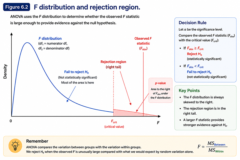
Figure 6.2. illustrates the F distribution and its right-tail rejection region. The precise location of the critical value depends on \(\alpha\), \(df_1\), and \(df_2\). The LearnerBox Statistical Explorer displays the observed F statistic and critical F value on the same reference distribution, allowing the numerical hypothesis test to be connected directly with the graphical decision region.
The results of an ANOVA are conventionally organised in an ANOVA table. The table summarises the partitioning of variability and shows how the F statistic is constructed. Although statistical software calculates the quantities automatically, understanding the structure of the table is essential for interpreting the model correctly.
A standard one-way ANOVA table has the following conceptual structure:
| Source | SS | df | MS | F | p |
|---|---|---|---|---|---|
| Between Groups | \(SS_{\text{Between}}\) | \(k-1\) | \(MS_{\text{Between}}\) | \(F\) | \(p\) |
| Within Groups | \(SS_{\text{Within}}\) | \(N-k\) | \(MS_{\text{Within}}\) | — | — |
| Total | \(SS_{\text{Total}}\) | \(N-1\) | — | — | — |
The Source column identifies the components of variation. Depending on the statistical software, the between-group source may be labelled with the actual factor name rather than the generic term Between Groups. For example, if Region is the factor, the first row may simply be labelled Region. The residual component may be labelled Within Groups, Error, or Residual.
The SS column contains the sums of squares associated with each source of variation. The df column shows the corresponding degrees of freedom, and the MS column contains the mean squares calculated by dividing each sum of squares by its degrees of freedom. The F statistic is obtained by dividing the factor mean square by the residual mean square.
For a one-way ANOVA:
\[ F = \frac{MS_{\text{Factor}}}{MS_{\text{Residual}}} \]The p-value in the factor row evaluates the omnibus null hypothesis. If \(p<\alpha\), the factor has a statistically significant omnibus effect on the dependent variable, meaning that the population means are not all equal. If \(p\geq\alpha\), the analysis provides insufficient statistical evidence to reject the equality of the population means.
The ANOVA table is more than a compact presentation of statistical output. It is a numerical representation of the model's variance-partitioning structure. The factor row represents variability systematically associated with group membership, the residual row represents unexplained within-group variability, and the F statistic compares the corresponding mean squares. Once this structure is understood, ANOVA output becomes considerably easier to interpret, even when additional factors and interaction terms are introduced in more complex models.
The one-way ANOVA table establishes whether there is statistically significant evidence of differences somewhere among the population means. However, statistical significance alone does not indicate the magnitude of the factor's association with the dependent variable, nor does a significant omnibus test identify which groups differ. These questions require effect-size measures and post hoc comparisons, which form the next stage of the ANOVA workflow.
This example examines whether mean Purchase Amount differs across geographical Regions. The omnibus ANOVA is not statistically significant. The example illustrates why post hoc comparisons are generally unnecessary when the overall model provides insufficient evidence of mean differences.
A customer analytics team wants to determine whether average Purchase Amount differs across the four geographical regions represented in the LearnerBox dataset. The research question is:
Does mean Purchase Amount differ across North, South, East, and West regions?
Because the dependent variable is continuous and the independent variable is a categorical factor containing four independent groups, a one-way ANOVA is appropriate.
The dependent variable is Purchase Amount, a continuous numerical variable. The factor is Region, which contains four levels: North, South, East, and West. Each customer belongs to only one region, so the groups are independent.
The null hypothesis states that the population mean Purchase Amount is equal across all four regions:
\[ H_0:\mu_{\text{North}} = \mu_{\text{South}} = \mu_{\text{East}} = \mu_{\text{West}} \]The alternative hypothesis is:
\[ H_1:\text{Not all regional population means are equal} \]The analysis will use a significance level of:
\[ \alpha=.05 \]The alternative hypothesis does not state that every regional mean must differ from every other regional mean. The omnibus ANOVA requires only sufficient evidence that the complete equality specified by \(H_0\) does not hold.
The first assumption is independence of observations. Each row in the dataset represents a separate customer, and each customer is classified into one Region. No customer contributes observations to multiple regional groups. The independence assumption is therefore supported by the structure of the data.
The normality assumption is assessed using the residuals from the ANOVA model. The LearnerBox Statistical Explorer reports the Shapiro-Wilk test for the model residuals. The null hypothesis of the Shapiro-Wilk test is that the residuals are normally distributed. The result should be interpreted together with the sample size and graphical evidence rather than as an automatic pass-or-fail rule.
Homogeneity of variance is assessed using Levene's test. The null hypothesis of Levene's test states that the population variances are equal across the regional groups. A non-significant result provides insufficient evidence that the variances differ and is therefore consistent with the homogeneity assumption.
The one-way ANOVA F statistic is:
\[ F = \frac{MS_{\text{Between}}}{MS_{\text{Within}}} \]where:
\[ MS_{\text{Between}} = \frac{SS_{\text{Between}}}{df_{\text{Between}}} \]and:
\[ MS_{\text{Within}} = \frac{SS_{\text{Within}}}{df_{\text{Within}}} \]The F-ratio therefore compares the variance estimate associated with regional differences with the residual variance estimate within the regional groups.
A complete manual ANOVA would require calculating the grand mean, four group means, squared deviations, three sums of squares, degrees of freedom, and mean squares. In an applied analysis, these quantities are obtained from statistical software. The important calculation is the construction of the F-ratio from the ANOVA table:
\[ F = \frac{MS_{\text{Region}}}{MS_{\text{Residual}}} \]The Explorer performs the complete variance partitioning and displays the sums of squares, degrees of freedom, mean squares, F statistic, and p-value in the ANOVA table.
Open the ANOVA tab in the LearnerBox Statistical Explorer. Select One-Way ANOVA, choose Region as the factor, and select Purchase Amount as the dependent variable. Use \(\alpha=.05\).
Begin with the grouped means and confidence intervals. The graph provides a descriptive comparison of the four regional means and the uncertainty surrounding each estimate. Next, examine the F-distribution graph. The observed F statistic is displayed relative to the critical F value and the right-tail rejection region.
The observed F statistic extends into the rejection region of the relevant F distribution. The ANOVA table reports:
\[ p\geq.05 \]The null hypothesis is therefore rejected. The data provide sufficient statistical evidence that mean Annual Income differs across the four regional populations.
Because the omnibus ANOVA is statistically significant, Tukey post hoc comparisons are not required to search for pairwise differences.
Numerical Result. The regional sample means show variation in average Purchase Amount. The ANOVA table partitions the total variability into a component associated with Region and a residual component within regions. The resulting F statistic is not sufficiently large to fall within the rejection region of the relevant F distribution.
Statistical Interpretation. The omnibus p-value is greater than \(\alpha=.05\). We fail to reject \(H_0\) and conclude that the population mean Purchase Amount is not different across all four regions. The non-significant result indicates that regional population means do not differ from another. Tukey-adjusted post hoc comparisons are therefore not conducted.
Practical Interpretation. The result suggests that geographical Region is not associated with variation in customer Purchase Amount. For the customer analytics team, regional differences may not be relevant to market segmentation, sales planning, or the design of region-specific customer strategies. The practical importance of the result should be interpreted together with the magnitude of the effect and the actual differences between the regional means.
A statistically non-significant one-way ANOVA establishes that the population means are similar. Therefore, post-hoc tests are not required.
This example examines whether mean Annual Income differs across geographical Regions. The analysis illustrates a statistically significant omnibus ANOVA and shows how post hoc comparisons are used to identify the group differences underlying the overall result.
A researcher wants to determine whether average Annual Income differs across the four geographical regions in the LearnerBox dataset. The research question is:
Does mean Annual Income differ across North, South, East, and West regions?
Annual Income is continuous and Region is a categorical factor with four independent levels. A one-way ANOVA is therefore appropriate.
The dependent variable is Annual Income. The factor is Region, with the levels North, South, East, and West. Each customer contributes one Annual Income observation and belongs to one regional group.
The null hypothesis is:
\[ H_0:\mu_{\text{North}} = \mu_{\text{South}} = \mu_{\text{East}} = \mu_{\text{West}} \]The alternative hypothesis is:
\[ H_1:\text{Not all regional population means are equal} \]The significance level is:
\[ \alpha=.05 \]The observations are treated as independent because each customer appears once in the analysis and belongs to one regional group. Residual normality is assessed using the Shapiro-Wilk test and the distribution of the model residuals. Homogeneity of variance is assessed using Levene's test.
The assumption results should be interpreted before the omnibus F-test. A non-significant Levene's test is consistent with approximately equal population variances. Similarly, the Shapiro-Wilk result should be considered together with the residual pattern and the robustness of ANOVA to moderate departures from normality.
The same one-way ANOVA F-ratio is used:
\[ F = \frac{MS_{\text{Region}}}{MS_{\text{Residual}}} \]The statistical procedure is unchanged from Worked Example 6.1. What changes is the relative magnitude of systematic and residual variation in the selected dependent variable.
The ANOVA table shows the variance components required to construct the F statistic. In this model, the variability associated with differences among the regional Annual Income means is not sufficiently large relative to the residual variability within the regions to produce a statistically significant omnibus result.
In the ANOVA tab, select One-Way ANOVA, choose Region as the factor, and select Annual Income as the dependent variable. Set the significance level to \(\alpha=.05\).
The grouped-means graph shows the sample mean Annual Income for each region with confidence intervals. Some numerical differences between the sample means are visible.
The ANOVA table provides the formal omnibus test. The p-value for Region is smaller than the selected significance level. Therefore:
\[ p<.05 \]The null hypothesis is rejected. There is statistically significant evidence that mean Annual Income is not equal across all four regions.
Because the omnibus ANOVA is statistically significant, the analysis proceeds to the Tukey post hoc comparisons. Each pairwise comparison should be evaluated using its adjusted p-value. Comparisons with an adjusted \(p<.05\) identify regional pairs for which there is statistically significant evidence of a difference in population mean Purchase Amount.
Numerical Result. The regional sample means show variation in average Annual Income. The ANOVA table partitions the total variability into a component associated with Region and a residual component within regions. The resulting F statistic is sufficiently large to fall within the rejection region of the relevant F distribution.
Statistical Interpretation. The omnibus p-value is smaller than \(\alpha=.05\). We reject \(H_0\) and conclude that the population mean Annual Income is not equal across all four regions. The significant result indicates that at least one regional population mean differs from another. Tukey-adjusted post hoc comparisons are then used to determine which regional differences are statistically significant.
Practical Interpretation. The result suggests that geographical Region is associated with variation in customer Annual Income. For the customer analytics team, regional differences may be relevant to market segmentation, sales planning, or the design of region-specific customer strategies. The practical importance of the result should be interpreted together with the magnitude of the effect and the actual differences between the regional means.
A non-significant ANOVA does not demonstrate that the population means are exactly equal. It indicates that the observed between-group variation is not sufficiently large relative to residual variation to reject the omnibus null hypothesis at the selected significance level.
The following exercises use the one-way ANOVA concepts developed in this part. Attempt each question before opening the answer.
A researcher compares mean Credit Score across four geographical regions using a one-way ANOVA. The analysis produces:
\[ F(3,96)=0.84,\quad p=.475 \]The significance level is \(\alpha=.05\). State the statistical decision and interpret the result.
Because \(p=.475\) is greater than \(\alpha=.05\), we fail to reject the null hypothesis. The analysis provides insufficient statistical evidence that population mean Credit Score differs across the four regions.
The result should not be interpreted as proof that all four population means are exactly equal. Instead, the observed between-region variation is not sufficiently large relative to within-region variation to produce a statistically significant omnibus F-test.
A one-way ANOVA compares mean customer Purchase Amount across four groups and produces:
\[ F(3,96)=7.42,\quad p<.001 \]Explain what can and cannot be concluded from the omnibus ANOVA result.
Because \(p<.001\), the p-value is smaller than \(\alpha=.05\), and the null hypothesis of equal population means is rejected. There is statistically significant evidence that the population mean Purchase Amount is not equal across all four groups.
The omnibus ANOVA establishes that at least one population mean differs from at least one other population mean. It does not identify the specific groups that differ and does not imply that every group differs from every other group. Appropriate post hoc comparisons, such as Tukey's procedure, should be examined to locate the statistically significant pairwise differences.
Two one-way ANOVA models produce the following results:
Model A:
\[ F(3,96)=1.12,\quad p=.345 \]Model B:
\[ F(3,96)=12.60,\quad p<.001 \]Both models use the same factor and contain the same number of observations. Explain what the difference in the F statistics suggests about between-group and within-group variation.
The F statistic is the ratio of the factor mean square to the residual mean square:
\[ F=\frac{MS_{\text{Between}}}{MS_{\text{Within}}} \]For Model A, \(F=1.12\). The between-group variance estimate is therefore only slightly larger than the within-group variance estimate. This pattern is broadly consistent with the null hypothesis, and the model is not statistically significant.
For Model B, \(F=12.60\). The between-group mean square is substantially larger relative to the within-group mean square. This indicates a much stronger systematic group component relative to residual variation and produces a statistically significant omnibus result.
The comparison demonstrates that the F statistic should be interpreted as a ratio of variance components. A large F value reflects stronger systematic variation associated with the factor relative to unexplained within-group variation.
A statistically significant ANOVA indicates that the observed pattern of group means is unlikely to be explained by sampling variation alone under the null hypothesis. Statistical significance, however, does not describe the magnitude of the effect. With a sufficiently large sample, even relatively small group differences may produce a small p-value. Conversely, a potentially meaningful pattern may fail to reach statistical significance when the sample provides limited precision or statistical power.
For this reason, ANOVA results should not be interpreted using the F statistic and p-value alone. An effect size quantifies the magnitude of the variation associated with a factor or model effect. It shifts the analytical question from:
Is there statistical evidence of a group effect?
to:
How much of the variability in the dependent variable is associated with the effect being studied?
This distinction reflects the four-layer interpretation framework used throughout LearnerBox. The p-value contributes to the statistical interpretation, whereas the effect size helps develop the practical interpretation. A complete ANOVA analysis should normally report both.
One of the most direct effect-size measures for ANOVA is eta squared, written as \(\eta^2\). Eta squared expresses the proportion of total variation in the dependent variable associated with a particular source of variation.
For a one-way ANOVA:
\[ \eta^2 = \frac{SS_{\text{Between}}}{SS_{\text{Total}}} \]More generally, the effect sum of squares may be written as \(SS_{\text{Effect}}\):
\[ \eta^2 = \frac{SS_{\text{Effect}}}{SS_{\text{Total}}} \]Because \(\eta^2\) is a proportion, its value ranges from 0 to 1. A value close to 0 indicates that the effect is associated with relatively little of the total variation in the dependent variable. A larger value indicates that a greater proportion of the observed variation is associated with the factor.
Suppose an ANOVA produces:
\[ SS_{\text{Between}}=2,400 \]and:
\[ SS_{\text{Total}}=20,000 \]Then:
\[ \eta^2 = \frac{2,400}{20,000} = 0.12 \]The factor is therefore associated with approximately 12% of the total observed variation in the dependent variable.
Conventional reference values are sometimes used to provide a broad description of effect magnitude:
\[ \eta^2\approx.01 \quad\text{Small} \] \[ \eta^2\approx.06 \quad\text{Medium} \] \[ \eta^2\approx.14 \quad\text{Large} \]These thresholds are interpretive conventions rather than universal laws. An effect considered small in one research context may have substantial practical importance in another. Effect size should therefore be interpreted in relation to the research question, measurement scale, previous research, and consequences of the observed difference.
In factorial ANOVA and other models containing multiple effects, researchers frequently report partial eta squared, written as partial \(\eta^2\). Partial eta squared measures the proportion of variation associated with a particular effect relative to that effect and the residual error variation.
The formula is:
\[ \eta_p^2 = \frac{SS_{\text{Effect}}} {SS_{\text{Effect}}+SS_{\text{Error}}} \]The subscript \(p\) indicates that the effect is being evaluated partially relative to its associated effect-plus-error variance. This becomes especially important in a two-way ANOVA, where the model may contain two main effects and an interaction effect.
For example, a two-way ANOVA containing Region and Loyalty Tier may include:
\[ \text{Region main effect} \] \[ \text{Loyalty Tier main effect} \] \[ \text{Region}\times\text{Loyalty Tier interaction} \]A separate partial \(\eta^2\) can be calculated for each effect. This allows the analyst to describe the magnitude of the Region effect, the Loyalty Tier effect, and the interaction effect separately.
Suppose the interaction has:
\[ SS_{\text{Interaction}}=800 \]and the model has:
\[ SS_{\text{Error}}=7,200 \]Then:
\[ \eta_p^2 = \frac{800}{800+7,200} = 0.10 \]The interaction accounts for approximately 10% of the effect-plus-error variance used in the partial effect-size calculation.
Eta squared and partial eta squared are therefore related but not interchangeable. Eta squared uses total variation in its denominator, whereas partial eta squared removes other model effects from the denominator and evaluates the selected effect relative to itself and residual error.
ANOVA is fundamentally concerned with differences among population means. The sample group means provide point estimates of those unknown population means, but a point estimate alone does not communicate the precision of the estimate. Confidence intervals for the group means provide an interval estimate around each sample mean.
The general structure remains:
\[ \text{Estimate} \pm \text{Critical Value}\times\text{Standard Error} \]For a group mean:
\[ \bar{x}_j \pm t^* \left( \frac{s_j}{\sqrt{n_j}} \right) \]where \(\bar{x}_j\) is the sample mean for group \(j\), \(s_j\) is the sample standard deviation, \(n_j\) is the group sample size, and \(t^*\) is the appropriate critical value.
The grouped-means graph in the LearnerBox Statistical Explorer displays the estimated mean for each group together with its confidence interval. This makes the graph useful for examining the pattern, direction, and precision of the group estimates before interpreting the formal inferential tests.
A narrow confidence interval indicates a more precise estimate of the group mean. A wider interval indicates greater uncertainty. Confidence interval width is influenced by the variability within the group, the group sample size, and the selected confidence level.
It is tempting to use overlap between individual group confidence intervals as a direct significance test. This should be avoided. The overlap of separate confidence intervals for two group means is not mathematically identical to a formal test of the difference between those means. The omnibus ANOVA and appropriately adjusted post hoc comparisons provide the inferential tests.
A statistically significant omnibus ANOVA indicates that the null hypothesis of equal population means is not supported. It does not, however, identify the particular groups responsible for the significant result. When a factor contains more than two levels, the analyst may therefore need to conduct post hoc tests.
The term post hoc means after this. In the ANOVA workflow, post hoc comparisons are typically examined after the omnibus F-test has established evidence of differences among the population means.
Suppose a one-way ANOVA compares four groups:
\[ A,\quad B,\quad C,\quad D \]The possible pairwise comparisons are:
\[ A-B,\quad A-C,\quad A-D,\quad B-C,\quad B-D,\quad C-D \]For \(k\) groups, the number of unique pairwise comparisons is:
\[ \frac{k(k-1)}{2} \]With four groups:
\[ \frac{4(4-1)}{2} = 6 \]Testing each pair using a separate unadjusted t-test would recreate the multiple-testing problem discussed earlier in this module. As the number of tests increases, the probability of making at least one Type I error across the family of comparisons also increases. Post hoc procedures address this problem by controlling or adjusting for multiple comparisons.
Tukey's Honestly Significant Difference test, commonly called Tukey's HSD, is designed for pairwise comparisons among group means following ANOVA. It evaluates all pairwise mean differences while controlling the familywise error rate.
The classical Tukey HSD criterion for equal group sizes is based on:
\[ HSD = q_{\alpha,k,df_{\text{Error}}} \sqrt{ \frac{MS_{\text{Error}}}{n} } \]where \(q\) is a critical value from the studentized range distribution, \(k\) is the number of groups, \(df_{\text{Error}}\) is the error degrees of freedom, \(MS_{\text{Error}}\) is the residual mean square, and \(n\) is the group sample size.
A pairwise mean difference is statistically significant when its magnitude is sufficiently large relative to the Tukey-adjusted comparison criterion. Modern statistical software also provides adjusted p-values and confidence intervals for the pairwise differences.
Tukey's HSD is particularly appropriate when the primary analytical objective is to compare every group with every other group. It provides a systematic set of pairwise comparisons and is the post hoc procedure displayed in the LearnerBox Statistical Explorer.
In the Explorer's post hoc table, the learner should examine the mean difference, the confidence interval, the adjusted p-value, and the resulting decision. The adjusted p-value—not an unadjusted pairwise p-value—is used for the statistical decision.
The Bonferroni adjustment provides a simple and general method for controlling the familywise error rate. If \(m\) statistical comparisons are performed, the overall significance level is divided by the number of comparisons:
\[ \alpha_{\text{Adjusted}} = \frac{\alpha}{m} \]Suppose six pairwise comparisons are conducted using an overall significance level of \(\alpha=.05\). The Bonferroni-adjusted significance level is:
\[ \alpha_{\text{Adjusted}} = \frac{.05}{6} = .0083 \]Each individual comparison would therefore need a p-value smaller than approximately .0083 to be declared statistically significant under this implementation of the adjustment.
An equivalent approach is to adjust the individual p-values:
\[ p_{\text{Adjusted}} = \min(mp,1) \]The adjusted p-value is then compared with the original significance level, such as \(\alpha=.05\).
The Bonferroni method is flexible because it can be applied to many families of statistical tests and is not restricted to all-pairs mean comparisons. Its main limitation is that it can be conservative, particularly when the number of comparisons is large. Stronger Type I error control may therefore be accompanied by reduced statistical power.
Scheffé's test is a highly conservative multiple-comparison procedure designed to protect the familywise error rate across a broad set of possible contrasts among group means. Unlike Tukey's HSD, its scope is not limited to pairwise comparisons.
A contrast may compare a weighted combination of population means:
\[ L = c_1\mu_1+c_2\mu_2+\cdots+c_k\mu_k \]subject to:
\[ \sum_{j=1}^{k}c_j=0 \]For example, a researcher may wish to compare the mean of one group with the combined mean of several other groups. Such a hypothesis is more complex than a simple pairwise comparison.
Scheffé's procedure provides protection across all possible contrasts that could be formed from the group means. This broad protection makes the procedure flexible, but it also makes Scheffé's test relatively conservative. A larger observed difference may be required to achieve statistical significance than under a procedure designed specifically for pairwise comparisons.
Scheffé's test is therefore particularly relevant when the analyst wishes to investigate complex or exploratory contrasts rather than only compare every pair of group means.
The appropriate multiple-comparison procedure depends on the inferential objective. Tukey's HSD is well suited to systematic all-pairs comparisons among group means. The Bonferroni adjustment is a flexible general method that can be applied to a selected family of comparisons but may become conservative as the number of tests increases. Scheffé's test offers broad protection for pairwise and complex contrasts but is generally more conservative.
These procedures should not be treated as interchangeable buttons that analysts select until a desired p-value appears. The comparison procedure should be chosen according to the research question and the family of inferences the researcher intends to make.
Tukey HSD: all pairwise comparisons.
Bonferroni: flexible adjustment for a defined family of tests.
Scheffé: broad protection for pairwise and complex contrasts.
A one-way ANOVA examines whether the population mean of a continuous dependent variable differs across the levels of one categorical factor. Many research questions, however, involve more than one factor. Customer behaviour may differ across geographical regions and loyalty tiers. Academic performance may vary according to teaching method and programme type. Employee productivity may be associated with both work arrangement and department. Analysing only one factor at a time may provide an incomplete representation of these relationships.
A two-way Analysis of Variance extends the ANOVA model by including two categorical factors. The term two-way refers to the presence of two factors in the model. It does not refer to a two-tailed hypothesis test.
Suppose Purchase Amount is analysed using Region and Loyalty Tier as factors. Region contains four levels:
\[ \text{North},\quad \text{South},\quad \text{East},\quad \text{West} \]and Loyalty Tier contains two levels:
\[ \text{VIP},\quad \text{Regular} \]Together, these factors define a factorial structure containing:
\[ 4\times2=8 \]combinations of factor levels. These combinations are called cells. For example, North–VIP, North–Regular, South–VIP, and South–Regular represent four of the eight cells in the design.
The two-way ANOVA does considerably more than conduct two separate one-way ANOVAs. A factorial model simultaneously evaluates three substantive effects:
1. The main effect of Factor A
2. The main effect of Factor B
3. The interaction between Factor A and Factor B
For two factors \(A\) and \(B\), the two-way ANOVA model can be expressed as:
\[ Y_{ijk} = \mu + \alpha_i + \beta_j + (\alpha\beta)_{ij} + \varepsilon_{ijk} \]In this model, \(Y_{ijk}\) is an observed value of the dependent variable, \(\mu\) is the grand mean, \(\alpha_i\) represents the effect associated with level \(i\) of Factor A, \(\beta_j\) represents the effect associated with level \(j\) of Factor B, \((\alpha\beta)_{ij}\) represents the interaction between the two factors, and \(\varepsilon_{ijk}\) represents residual variation.
The total variation is therefore partitioned into four components:
\[ SS_{\text{Total}} = SS_A + SS_B + SS_{A\times B} + SS_{\text{Error}} \]This partitioning is the central advantage of factorial ANOVA. Instead of examining each factor in isolation, the model estimates the variation associated with each factor and with their joint relationship while retaining a residual error component.
A main effect evaluates the association between one factor and the dependent variable while averaging across the levels of the other factor. In a two-way ANOVA containing Factors \(A\) and \(B\), the model contains a main effect for \(A\) and a separate main effect for \(B\).
Consider a model in which Purchase Amount is the dependent variable and Region and Loyalty Tier are the factors. The main effect of Region evaluates whether mean Purchase Amount differs across geographical regions when the Loyalty Tier levels are averaged together.
Conceptually, the regional means used for the main effect are marginal means. For example, the mean for the North region is based on the Purchase Amount values for North–VIP and North–Regular customers considered across Loyalty Tier.
The null hypothesis for the Region main effect is:
\[ H_{0A}: \mu_{\text{North}} = \mu_{\text{South}} = \mu_{\text{East}} = \mu_{\text{West}} \]The alternative hypothesis is:
\[ H_{1A}: \text{Not all regional marginal means are equal} \]The main effect of Loyalty Tier asks a different question. It evaluates whether mean Purchase Amount differs between VIP and Regular customers when the Region levels are averaged together.
The corresponding null hypothesis is:
\[ H_{0B}: \mu_{\text{VIP}} = \mu_{\text{Regular}} \]The alternative hypothesis is:
\[ H_{1B}: \mu_{\text{VIP}} \neq \mu_{\text{Regular}} \]Each main effect has its own sum of squares, degrees of freedom, mean square, F statistic, p-value, and effect-size estimate. For Factor \(A\):
\[ F_A = \frac{MS_A}{MS_{\text{Error}}} \]For Factor \(B\):
\[ F_B = \frac{MS_B}{MS_{\text{Error}}} \]The denominator is the residual mean square in both tests. The numerator changes according to the effect being evaluated.
For a factor containing \(a\) levels:
\[ df_A=a-1 \]For a factor containing \(b\) levels:
\[ df_B=b-1 \]Thus, in a \(4\times2\) Region by Loyalty Tier design:
\[ df_{\text{Region}}=4-1=3 \]and:
\[ df_{\text{Loyalty Tier}}=2-1=1 \]It is possible for one main effect to be statistically significant while the other is not. For example, Purchase Amount may differ substantially between VIP and Regular customers but show little overall variation across Region. The ANOVA table evaluates these effects separately.
The most distinctive feature of a factorial ANOVA is its ability to evaluate an interaction effect. An interaction occurs when the effect of one factor on the dependent variable depends on the level of another factor.
For Factors \(A\) and \(B\), the interaction is written as:
\[ A\times B \]The null hypothesis for the interaction is:
\[ H_{0AB}: \text{There is no interaction between Factors }A\text{ and }B \]The alternative hypothesis is:
\[ H_{1AB}: \text{There is an interaction between Factors }A\text{ and }B \]Consider again the Region by Loyalty Tier analysis of Purchase Amount. Suppose VIP customers have a higher mean Purchase Amount than Regular customers in every region and the size of this difference is approximately constant. Loyalty Tier may have a main effect, but the pattern does not suggest a strong interaction. The relationship between Loyalty Tier and Purchase Amount is broadly similar across Region.
Now suppose the VIP–Regular difference is small in the North, moderate in the South, large in the East, and reversed in the West. The effect of Loyalty Tier is no longer consistent across geographical regions. The relationship between Loyalty Tier and Purchase Amount depends on Region. This is an interaction.
The F statistic for the interaction is:
\[ F_{A\times B} = \frac{MS_{A\times B}}{MS_{\text{Error}}} \]The interaction degrees of freedom are:
\[ df_{A\times B} = (a-1)(b-1) \]For a \(4\times2\) factorial design:
\[ df_{A\times B} = (4-1)(2-1) = 3 \]The interaction term therefore evaluates whether the pattern of cell means contains systematic variation beyond the additive main effects of the two factors.
An interaction plot provides a visual representation of this pattern. The levels of one factor are placed on the horizontal axis, while separate lines represent the levels of the second factor. The vertical axis displays the mean of the dependent variable.
When the lines are approximately parallel, the difference between the levels represented by the lines remains broadly consistent across the horizontal-axis factor. This pattern is consistent with little or no interaction.
When the lines are clearly non-parallel, the size of the difference changes across factor levels. The lines may converge, diverge, or cross. Such patterns provide visual evidence of a possible interaction.
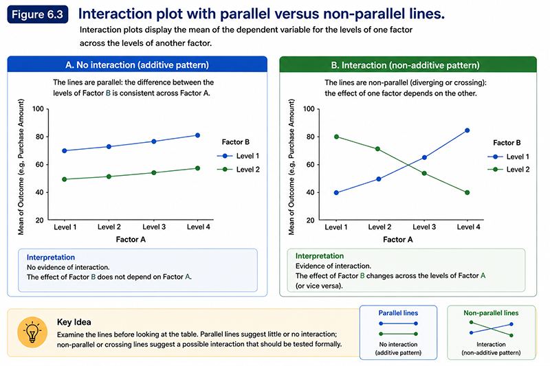
Figure 6.3. Interaction plot with parallel versus non-parallel lines.
The interaction plot is a descriptive diagnostic and should not replace the formal F-test for the interaction term. Slightly non-parallel lines can occur because of sampling variability, while a statistically significant interaction may sometimes appear visually modest depending on the graph scale and sample precision. The interaction p-value in the ANOVA table provides the formal inferential test.
A two-way ANOVA should be interpreted as a factorial model rather than as three unrelated hypothesis tests. The main effects and interaction describe different components of the same pattern of cell means. The order in which the model is interpreted is therefore important.
The first step is to examine the interaction effect. If the interaction is statistically significant, the relationship between one factor and the dependent variable differs across the levels of the other factor. In this situation, the marginal means underlying the main effects may conceal important differences in the cell-level pattern.
For example, suppose the overall mean Purchase Amount is higher for VIP customers than for Regular customers. This suggests a Loyalty Tier main effect. However, imagine that VIP customers spend substantially more in the North and East, show almost no difference in the South, and spend less than Regular customers in the West. The average VIP–Regular difference may still be positive, but that marginal mean difference does not adequately describe the conditional pattern.
When a statistically significant interaction is present, the analyst should therefore interpret the interaction carefully and examine the relevant cell means, interaction plot, and appropriate follow-up comparisons. The question becomes:
How does the effect of one factor differ across the levels of the other factor?
These conditional comparisons are often described as simple effects or simple main effects. For example, the analyst may examine the effect of Loyalty Tier separately within each Region or compare Regions separately for VIP and Regular customers.
If the interaction is not statistically significant, the main effects can generally be interpreted more directly. The analyst examines the F statistic and p-value for Factor A and then for Factor B. A significant main effect indicates evidence of differences among the marginal population means for that factor.
The ANOVA table for a two-way model therefore contains separate substantive rows for:
\[ \text{Factor A} \] \[ \text{Factor B} \] \[ \text{Factor A}\times\text{Factor B} \]Each row should be read across to identify the degrees of freedom, mean square, F statistic, p-value, and partial \(\eta^2\). The residual row provides the error variance used as the denominator for the three F-ratios.
A useful interpretation sequence is:
1. Examine the interaction plot and cell means.
Understand the observed factorial pattern before reducing it to hypothesis-test decisions.
2. Interpret the interaction F-test.
Determine whether there is statistical evidence that the effect of one factor depends on the other factor.
3. If the interaction is significant, prioritise the interaction.
Examine the conditional pattern and appropriate simple effects. Main effects should be interpreted cautiously because marginal means may obscure the interaction.
4. If the interaction is not significant, interpret the main effects.
Evaluate whether the marginal population means differ across the levels of Factor A and Factor B.
5. Examine effect sizes.
Use partial \(\eta^2\) to evaluate the magnitude of each model effect rather than relying on p-values alone.
6. Conduct follow-up comparisons when required.
For factors containing more than two levels, adjusted comparisons may be needed to identify specific differences among marginal means or to investigate a significant interaction.
Consider three possible model patterns. In the first, neither main effect nor the interaction is statistically significant. The analysis provides insufficient evidence of systematic mean differences associated with either factor or their combination. In the second, one or both main effects are significant but the interaction is not. The factors show additive associations with the dependent variable, and the marginal means can be interpreted relatively directly.
The third pattern is the most analytically interesting: the interaction is statistically significant. Here, the effect of one factor varies across the levels of the other factor. The model can no longer be summarised adequately by saying simply that “Factor A has an effect” or “Factor B has an effect.” The analyst must describe the conditional structure of the relationship.
This distinction between additive and conditional effects is fundamental to statistical modelling. As the models become more advanced, the same reasoning will reappear in regression through interaction terms, moderation, and models containing multiple predictors. Two-way ANOVA therefore introduces a much broader analytical principle: the relationship between a predictor and an outcome may depend on context.
The analysis investigates whether mean Annual Income differs across the levels of two categorical factors, education and region, and whether the effect of one factor depends on the level of the other factor. The research question therefore contains three related components: whether Factor A has a main effect, whether Factor B has a main effect, and whether an \(A\times B\) interaction is present.
The dependent variable is Income, measured as a continuous outcome. Factor A is Education, consisting of five levels (High School, Diploma, Graduate, Bachelor, and Post Graduate). Factor B is Region, consisting of four levels. Each participant belongs to one education level and one region, forming the cells of the factorial design.
The complete design contains:
\[ 5\times4=20 \]cells, where \(a=5\) is the number of levels of Education and \(b=4\) is the number of levels of Region.
The first null hypothesis evaluates the marginal means of Education:
\[ H_{0A}: \mu_{\text{High School}} = \mu_{\text{Diploma}} = \mu_{\text{Graduate}} = \mu_{\text{Bachelor}} = \mu_{\text{Post Graduate}} \]The alternative hypothesis is:
\[ H_{1A}: \text{Not all marginal means of Education are equal} \]The second null hypothesis evaluates the marginal means of Region:
\[ H_{0B}: \mu_{R1} = \mu_{R2} = \mu_{R3} = \mu_{R4} \]The alternative hypothesis is:
\[ H_{1B}: \text{Not all marginal means of Region are equal} \]The interaction hypotheses are:
\[ H_{0AB}: \text{There is no interaction between Education and Region} \] \[ H_{1AB}: \text{The effect of Education depends on Region} \]The significance level is:
\[ \alpha=.05 \]The dependent variable is continuous, and the two predictors are categorical factors. Independence is assumed from the study design, with each observation contributing to only one Education × Region combination.
Normality was assessed using the residuals from the complete factorial model. The Shapiro–Wilk test was statistically significant (\(W=0.793,\ p<.0001\)), indicating evidence that the residuals deviate from normality.
Homogeneity of variance was assessed using Levene's test across the factorial cells. The test was not statistically significant (\(F=0.971,\ p=0.4985\)), indicating that the assumption of equal variances was satisfied.
The design contained 150 observations distributed across 20 cells, providing adequate data for estimation of the factorial model.
The two-way ANOVA model is:
\[ Y_{ijk} = \mu + \alpha_i + \beta_j + (\alpha\beta)_{ij} + \varepsilon_{ijk} \]Total variability is partitioned as:
\[ SS_{\text{Total}} = SS_A + SS_B + SS_{A\times B} + SS_{\text{Error}} \]Each substantive effect has its own F-ratio:
\[ F_A = \frac{MS_A}{MS_{\text{Error}}} \] \[ F_B = \frac{MS_B}{MS_{\text{Error}}} \] \[ F_{A\times B} = \frac{MS_{A\times B}}{MS_{\text{Error}}} \]The LearnerBox Statistical Explorer performs the complete variance partitioning. The essential manual step is to recognise how each F statistic is constructed from the ANOVA table. For example, the interaction statistic is:
\[ F_{A\times B} = \frac{ SS_{A\times B}/df_{A\times B} }{ SS_{\text{Error}}/df_{\text{Error}} } \]Substituting the values from the ANOVA table:
\[ F = \frac{1295984380.641/12} {33769968323.111/130} = \frac{107998698.387} {259768987.101} = 0.416 \]The interaction degrees of freedom are:
\[ df_{A\times B} = (5-1)(4-1)=12 \]The partial effect size for each term is:
\[ \eta_p^2 = \frac{SS_{\text{Effect}}} {SS_{\text{Effect}}+SS_{\text{Error}}} \]For the interaction, \[ \eta_p^2=0.037. \]
Select the two-way ANOVA model shown in the Explorer. Inspect the grouped means, confidence intervals, and ANOVA table. Because the interaction is not statistically significant, the main effects can be interpreted directly without considering conditional simple effects.
The ANOVA table produced the following results:
Because the interaction p-value (\(0.9552\)) is greater than \(\alpha=.05\), the null hypothesis of no interaction is not rejected. This indicates that the effect of Education on Income is consistent across the different Regions.
Numerical Result. The Education × Region interaction was not statistically significant, \(F(12,130)=0.416,\ p=0.9552,\ \eta_p^2=0.037\). Education showed a statistically significant main effect on Income, \(F(4,130)=7.754,\ p<.0001,\ \eta_p^2=0.193\), whereas Region did not have a statistically significant main effect, \(F(3,130)=1.648,\ p=0.1814,\ \eta_p^2=0.037\).
Statistical Interpretation. The non-significant interaction indicates that the relationship between Education and Income does not differ across Regions. Therefore, the main effects can be interpreted directly. Education significantly influences Income, whereas Region does not explain a statistically significant proportion of the variation in Income.
Practical Interpretation. Income differs across educational attainment regardless of geographic region. Individuals with higher educational qualifications generally earn different incomes than those with lower qualifications, while regional differences are comparatively small after accounting for education. Because no interaction was detected, the influence of Education appears stable across all Regions.
When the interaction is not statistically significant, the effects of the two factors are interpreted as additive rather than conditional. The main effects therefore provide the primary substantive conclusions. In this example, Education has a statistically significant effect on Income, whereas Region does not, and the influence of Education is consistent across Regions.
The analysis investigates whether mean bank savings balance differs across the levels of two categorical factors, location and employment status, and whether the effect of one factor depends on the level of the other factor. The research question therefore contains three related components: whether Factor A has a main effect, whether Factor B has a main effect, and whether an \(A\times B\) interaction is present.
The dependent variable is Savings Balance, measured as a continuous outcome. Factor A is Employment Status, consisting of two levels (Unemployed and Employed). Factor B is Location, consisting of two levels (Rural and Urban). Each participant belongs to one employment status and one location, forming the cells of the factorial design.
The complete design contains:
\[ 2\times2=4 \]cells, where \(a=2\) is the number of levels of Employment Status and \(b=2\) is the number of levels of Location.
The first null hypothesis evaluates the marginal means of Employment Status:
\[ H_{0A}: \mu_{\text{Unemployed}} = \mu_{\text{Employed}} \]The alternative hypothesis is:
\[ H_{1A}: \mu_{\text{Unemployed}} \neq \mu_{\text{Employed}} \]The second null hypothesis evaluates the marginal means of Location:
\[ H_{0B}: \mu_{\text{Rural}} = \mu_{\text{Urban}} \]The alternative hypothesis is:
\[ H_{1B}: \mu_{\text{Rural}} \neq \mu_{\text{Urban}} \]The interaction hypotheses are:
\[ H_{0AB}: \text{There is no interaction between Employment Status and Location} \] \[ H_{1AB}: \text{The effect of Employment Status depends on Location} \]The significance level is:
\[ \alpha=.05 \]The dependent variable is continuous, and the two predictors are categorical factors. Independence is assumed from the study design, with each observation contributing to only one Employment Status × Location combination.
Normality was assessed using the residuals from the complete factorial model. The Shapiro–Wilk test was not statistically significant (\(W=0.987,\ p=0.1919\)), indicating that the residuals do not depart significantly from normality.
Homogeneity of variance was assessed using Levene's test across the factorial cells. The test was not statistically significant (\(F=0.519,\ p=0.6695\)), indicating that the assumption of equal variances was satisfied.
The design contained 150 observations distributed across 4 cells, providing adequate data for estimation of the factorial model.
The two-way ANOVA model is:
\[ Y_{ijk} = \mu + \alpha_i + \beta_j + (\alpha\beta)_{ij} + \varepsilon_{ijk} \]Total variability is partitioned as:
\[ SS_{\text{Total}} = SS_A + SS_B + SS_{A\times B} + SS_{\text{Error}} \]Each substantive effect has its own F-ratio:
\[ F_A = \frac{MS_A}{MS_{\text{Error}}} \] \[ F_B = \frac{MS_B}{MS_{\text{Error}}} \] \[ F_{A\times B} = \frac{MS_{A\times B}}{MS_{\text{Error}}} \]The LearnerBox Statistical Explorer performs the complete variance partitioning. The essential manual step is to recognise how each F statistic is constructed from the ANOVA table. For example, the interaction statistic is:
\[ F_{A\times B} = \frac{ SS_{A\times B}/df_{A\times B} }{ SS_{\text{Error}}/df_{\text{Error}} } \]Substituting the values from the ANOVA table:
\[ F = \frac{853530395.070/1} {167184626.085/146} = \frac{853530395.070} {1145097.042} = 74.538 \]The interaction degrees of freedom are:
\[ df_{A\times B} = (2-1)(2-1)=1 \]The partial effect size for each term is:
\[ \eta_p^2 = \frac{SS_{\text{Effect}}} {SS_{\text{Effect}}+SS_{\text{Error}}} \]For the interaction,
\[ \eta_p^2=0.338. \]Select the significant two-way model shown in the Explorer. Begin with the grouped cell means and confidence intervals, then examine the interaction plot. The clearly non-parallel lines indicate that the relationship between employment status and savings balance changes across the two locations.
The ANOVA table produced the following results:
Because the interaction p-value is smaller than \(\alpha=.05\), the null hypothesis of no interaction is rejected. The effect of employment status on savings balance differs according to whether participants live in rural or urban locations.
Numerical Result. The Employment Status × Location interaction was statistically significant, \(F(1,146)=74.538,\ p<.0001,\ \eta_p^2=0.338\). Employment Status also had a statistically significant main effect, \(F(1,146)=209.064,\ p<.0001,\ \eta_p^2=0.589\), and Location showed a statistically significant main effect, \(F(1,146)=351.552,\ p<.0001,\ \eta_p^2=0.707\).
Statistical Interpretation. The significant interaction indicates that Employment Status and Location do not operate independently in influencing savings balance. The increase in savings associated with being employed is substantially greater for individuals living in urban areas than for those living in rural areas. Consequently, the interaction should be interpreted before considering the overall main effects.
Practical Interpretation. Employment is associated with higher savings balances in both rural and urban locations; however, the financial advantage of being employed is much larger in urban areas. This suggests that the benefits of employment on accumulated savings depend on where individuals live, highlighting the importance of considering both factors together rather than separately.
When an interaction is statistically significant, the effects are conditional rather than purely additive. The interaction plot demonstrates that the effect of Employment Status on Savings Balance depends on Location. Consequently, interpretation should focus first on the interaction and the corresponding subgroup patterns before drawing conclusions from the overall main effects.
Attempt each exercise before revealing the answer.
A two-way ANOVA examines examination scores by Teaching Method and Programme Type. The interaction result is:
\[ F(2,114)=5.24,\quad p=.007,\quad \eta_p^2=.084 \]Interpret the interaction and explain how it affects the interpretation of the main effects.
Because \(p=.007<.05\), the no-interaction null hypothesis is rejected. There is statistically significant evidence that the effect of Teaching Method on examination scores depends on Programme Type.
The partial effect size, \(\eta_p^2=.084\), indicates that approximately 8.4% of the interaction-plus-error variance is associated with the interaction term. Using conventional guidelines, this is approximately a medium effect.
Because the interaction is significant, the marginal main effects should not be interpreted in isolation. The analyst should examine the cell means, interaction plot, and simple effects of Teaching Method within each Programme Type, or Programme Type within each Teaching Method.
A factorial ANOVA produces the following results:
Describe the model pattern.
Factor A has a statistically significant main effect because \(p=.003<.05\). Factor B also has a statistically significant main effect because \(p=.003<.05\). The interaction is not statistically significant because \(p=.542>.05\).
The results therefore support an additive pattern. The marginal means differ across Factor A and across Factor B, but there is insufficient evidence that the effect of one factor changes across the levels of the other factor.
Because Factor A contains more than two levels, adjusted comparisons may be required to determine which marginal means differ. Factor B contains two levels, so its main effect directly represents the difference between those two marginal means.
An interaction plot shows two crossing lines, but the ANOVA table reports:
\[ F(2,54)=1.31,\quad p=.278 \]What conclusion should be reached?
The crossing lines describe the pattern observed in the sample, but the formal interaction test is not statistically significant because \(p=.278>.05\). The no-interaction null hypothesis is therefore not rejected.
There is insufficient statistical evidence that the apparent crossing pattern represents a population interaction rather than sampling variation. The plot should be used to understand the descriptive pattern, but it should not override the interaction F-test.
Selecting an appropriate mean-comparison procedure depends on the research question, the number of categorical factors, the number and relationship of the groups or measurements, and whether the analysis concerns a single benchmark, two means, or a broader factorial structure. The methods covered in Modules 5 and 6 belong to the same general family of parametric procedures, but they address different designs. The correct choice should therefore follow from the structure of the study rather than from the statistical result the researcher expects or hopes to obtain.
A t-test is appropriate when the research question concerns one mean, one mean difference, or a comparison between two means. A one-sample t-test compares a sample mean with a hypothesised population value. An independent-samples t-test compares the population means of two unrelated groups, while a paired-samples t-test evaluates the mean difference between two related measurements or matched observations. When an independent factor contains only two levels, the independent-samples t-test and the corresponding one-way ANOVA produce equivalent omnibus conclusions:
\[ F=t^2 \]This equivalence reflects the shared statistical logic of the two procedures. The t-test expresses the mean difference relative to its standard error, whereas ANOVA expresses model-associated variation relative to residual variation. With two groups, these approaches lead to the same p-value for the non-directional hypothesis. Nevertheless, the t-test is generally more direct because it reports the direction of the mean difference and aligns naturally with a research question involving exactly two groups.
A one-way ANOVA is appropriate when one categorical factor is used to compare the mean of a continuous dependent variable across three or more independent groups. For example, Region may contain North, South, East, and West levels, while Purchase Amount is the continuous outcome. The omnibus F-test evaluates whether the corresponding population means are all equal. If the omnibus result is significant, effect size and appropriate follow-up comparisons are used to determine the magnitude and location of the differences.
A two-way ANOVA is appropriate when the model contains two categorical factors and one continuous dependent variable. It simultaneously evaluates the main effect of each factor and the interaction between them. This design is selected not merely because the dataset contains two categorical variables, but because the research question concerns their separate and joint associations with the outcome. For example, a researcher may investigate whether Purchase Amount differs by Region, whether it differs by Loyalty Tier, and whether the effect of Loyalty Tier depends on Region.
The distinction between independent and related observations remains essential. One-way and two-way ANOVA, as developed in this module, assume a between-subjects design in which each case contributes one observation to one group or factorial cell. If the same participants are measured repeatedly across three or more conditions, a standard one-way between-subjects ANOVA is inappropriate. Such data require a repeated-measures ANOVA or another model that accounts for dependence among observations.
A practical decision sequence begins by identifying the inferential objective. If one sample mean is compared with a benchmark and the population standard deviation is unknown, use a one-sample t-test. If two independent group means are compared, use an independent-samples t-test, with Welch's procedure providing a reliable default. If two related measurements are compared, use a paired-samples t-test. If one factor contains three or more independent levels, use a one-way ANOVA. If two categorical factors are analysed simultaneously and interaction is substantively relevant, use a two-way ANOVA.
| Research Design | Appropriate Procedure | Primary Inferential Question |
|---|---|---|
| One sample compared with a benchmark | One-sample t-test | Does the population mean differ from the hypothesised value? |
| Two independent groups | Independent-samples t-test | Do the two population means differ? |
| Two related measurements or matched pairs | Paired-samples t-test | Does the population mean difference differ from zero? |
| One factor with three or more independent levels | One-way ANOVA | Are the population means all equal across the factor levels? |
| Two categorical factors | Two-way ANOVA | Are there main effects, and is there an interaction? |
The choice between one-way and two-way ANOVA should also reflect the theoretical model. Conducting separate one-way ANOVAs for two factors does not reproduce a two-way analysis because separate models cannot estimate the interaction between the factors. They may also attribute variation differently because each factor is analysed without accounting for the other. A factorial ANOVA is therefore required when the objective is to estimate both main effects and their conditional relationship within one coherent model.
Figure 6.4 summarises this decision process. The flowchart begins with the number of means or measurements being compared, then distinguishes independent from related observations and one-factor from two-factor designs. The figure should be used as a test-selection guide rather than as a substitute for understanding the research design.
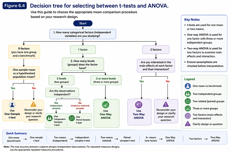
This module extended the mean-comparison framework from t-tests to Analysis of Variance. The transition became necessary because a series of unadjusted pairwise t-tests does not provide an appropriate omnibus analysis of several population means and inflates the familywise Type I error rate. ANOVA addresses this problem by evaluating all means represented by a factor within a single model before any follow-up comparisons are considered.
The central mathematical principle of ANOVA is variance partitioning. Total variation in the dependent variable is separated into systematic variation associated with the factors in the model and residual variation among observations within groups or cells. Sums of squares quantify these components, degrees of freedom convert them into mean squares, and the F statistic compares the relevant effect mean square with the residual mean square:
\[ F= \frac{MS_{\text{Effect}}}{MS_{\text{Error}}} \]The one-way ANOVA examined one categorical factor and tested the omnibus null hypothesis that all corresponding population means were equal. A significant F-test established that the means were not all equal, but did not identify which groups differed. Tukey's HSD, the Bonferroni adjustment, and Scheffé's procedure were introduced as methods for controlling familywise error during follow-up inference. Their suitability depends on whether the objective is to examine all pairwise comparisons, a defined family of tests, or a broader set of complex contrasts.
Effect sizes extended the interpretation beyond the omnibus p-value. Eta squared, \(\eta^2\), described the proportion of total observed variation associated with an effect, while partial eta squared, \(\eta_p^2\), evaluated an effect relative to that effect and residual error. Confidence intervals for group means supplemented these results by communicating the precision of the estimated means, although overlap between separate intervals was not treated as a substitute for formal pairwise inference.
The two-way ANOVA expanded variance partitioning to a factorial model containing two main effects and an interaction. Main effects described differences among marginal means, whereas the interaction tested whether the effect of one factor depended on the level of the other. When an interaction was significant, interpretation shifted from overall marginal patterns to cell means, interaction plots, and conditional comparisons. When the interaction was not significant, the main effects could generally be interpreted more directly as additive components of the model.
Across the worked examples, the LearnerBox Statistical Explorer connected descriptive patterns with inferential evidence. Grouped means and confidence intervals displayed the observed structure, the F-distribution graph located the test statistic relative to the rejection region, the ANOVA table showed the variance partitioning, post hoc output identified adjusted pairwise differences, and partial effect sizes described the magnitude of factorial effects. Significant and non-significant models were both treated as valid analytical outcomes requiring careful interpretation.
The complete ANOVA workflow can therefore be summarised as:
Define the factorial design → assess assumptions → partition the variability → construct the F-ratios → interpret the omnibus effects → quantify effect magnitude → conduct justified follow-up comparisons → interpret the model in context → report the findings.
Total Variation → Systematic Effects + Interaction Effects + Residual Variation
The F-test determines whether the systematic component is sufficiently large relative to residual error, while effect sizes and follow-up comparisons explain the magnitude and structure of the result.
Take a short quiz and find your score. You can always return to this page and review the content again.