

If you find the content useful and wish to support our platform’s development, you can contribute any amount toward our production costs. Scan the UPI QR code for payment within India. Or use the Ko-fi link to process a secure payment via PayPal.
If you find the content useful and wish to support our platform’s development, you can contribute any amount toward our production costs. Scan the UPI QR code for payment within India. Or use the Ko-fi link to process a secure payment via PayPal.
In the previous module, we learned how probability distributions describe uncertainty and how confidence intervals allow us to estimate unknown population parameters from sample data. However, many research questions require more than estimation. Researchers often wish to determine whether an observed difference is large enough to be considered statistically meaningful or whether it could simply have occurred because of random sampling variation.
Statistical hypothesis testing provides a systematic framework for answering these questions. Rather than relying on intuition or subjective judgement, hypothesis tests use probability theory to evaluate the strength of evidence contained within sample data. This enables researchers to make objective decisions about claims concerning populations while acknowledging that every conclusion is accompanied by some degree of uncertainty.
Hypothesis testing is one of the most widely used techniques in applied statistics. It underpins research across medicine, psychology, education, engineering, business, economics, artificial intelligence, and countless other disciplines. Whether evaluating the effectiveness of a new drug, comparing student performance before and after an educational intervention, assessing customer satisfaction following a marketing campaign, or determining whether a machine-learning algorithm improves prediction accuracy, the underlying statistical reasoning follows the same fundamental principles.
It is important to recognise what hypothesis testing does not do. A statistical test never proves that a hypothesis is true. Instead, it evaluates whether the observed data would be reasonably expected if the null hypothesis were correct. If the observed evidence appears highly unlikely under the null hypothesis, we reject it in favour of an alternative explanation. If the evidence is not sufficiently strong, we simply conclude that there is insufficient evidence to reject the null hypothesis.
This distinction may appear subtle, but it lies at the heart of statistical reasoning. Throughout this module, you will repeatedly encounter situations where the correct conclusion is not that the null hypothesis has been proven, but rather that the available evidence is either strong enough or not strong enough to justify rejecting it.
After successfully completing this module, you should be able to:
Data collected from samples almost never produce identical results. Two samples drawn from the same population will naturally differ because of random variation. For example, if two researchers independently survey 100 customers regarding their satisfaction with an online shopping experience, the average satisfaction scores are unlikely to be exactly the same, even if both samples were drawn from an identical customer population. Similarly, two clinical trials evaluating the same medication may report slightly different treatment effects, and two schools implementing the same teaching strategy may observe different average examination scores.
This natural variability presents an important challenge. When we observe a difference between groups or between a sample and a known value, how can we determine whether the difference reflects a genuine underlying effect or is merely the result of random chance? Visual inspection alone cannot provide a reliable answer. Small differences may appear meaningful even though they arise naturally from sampling variation, while genuinely important effects may appear modest because of variability within the data.
Statistical hypothesis testing addresses this problem by providing an objective decision-making framework grounded in probability theory. Instead of asking whether two values are exactly equal—which is rarely the case in real-world data—we ask whether the observed difference is sufficiently large that it would be unlikely to occur if the null hypothesis were true. Probability therefore becomes a tool for evaluating evidence rather than certainty.
This approach explains why hypothesis testing is often described as the bridge between descriptive statistics and inferential statistics. Descriptive statistics summarise the characteristics of a sample, while hypothesis testing allows researchers to draw carefully justified conclusions about the wider population from which that sample was obtained.
Modern research increasingly emphasises that statistical significance should never be interpreted in isolation. A complete statistical analysis considers the size of the observed effect, the confidence interval surrounding the estimate, the practical importance of the findings, and the broader context of the research question. Throughout this module, you will learn to interpret hypothesis tests using all of these perspectives rather than relying solely on whether a p-value is smaller than 0.05.
In Module 4, we learned that samples provide valuable information about populations, but they also contain unavoidable random variation. Using probability theory, we studied sampling distributions, the Central Limit Theorem, standard errors, confidence intervals, and statistical inference. Together, these concepts enabled us to estimate unknown population parameters while quantifying the uncertainty associated with those estimates.
Confidence intervals represented an important milestone because they shifted our focus from individual sample values to plausible ranges of population values. Rather than asking for a single "correct" estimate, we acknowledged that every estimate obtained from a sample is subject to sampling variability. The confidence interval therefore provided a range of values that are consistent with the observed data at a specified level of confidence.
However, estimation is only one aspect of statistical inference. Researchers are often interested in making decisions rather than simply estimating parameters. Consider the following questions:
These questions require more than estimating a population mean. They require us to evaluate evidence and determine whether the observed differences are sufficiently large that they are unlikely to have arisen through random sampling variation alone. This transition from estimation to formal decision making marks the beginning of statistical hypothesis testing.
An important connection exists between the two approaches. As you will discover later in this module, confidence intervals and hypothesis tests are not separate statistical techniques. They represent two different ways of answering the same inferential question. A confidence interval provides a range of plausible population values, while a hypothesis test evaluates whether a particular hypothesised value remains plausible in light of the observed evidence. Understanding this relationship is one of the key conceptual goals of this module.
The methods introduced in this chapter form the foundation of almost every statistical procedure that follows. Analysis of variance, regression modelling, and many machine learning algorithms all rely on the same principles of statistical inference introduced here. Learning to formulate hypotheses, evaluate evidence, and interpret results correctly is therefore an essential step towards more advanced data analysis. By the end of this module, you will be able to move confidently from a research question to a statistical conclusion. More importantly, you will understand why each decision is made, enabling you to interpret statistical results critically rather than simply applying formulas mechanically. This way of thinking forms the foundation for more advanced statistical methods such as analysis of variance, regression modelling, machine learning, and predictive analytics, all of which build upon the same principles of statistical inference introduced here.
The word hypothesis simply refers to a statement or claim that can be investigated using evidence. In everyday life, people frequently make hypotheses, often without realising it. For example, someone may believe that a new teaching method improves examination performance, that customers spend more after joining a loyalty programme, or that a redesigned website increases online purchases. These are all hypotheses because they make claims about the world that can be evaluated using data.
In statistics, however, hypotheses are defined much more precisely. A statistical hypothesis is a statement about one or more characteristics of a population, usually expressed in terms of population parameters such as the population mean (μ), population proportion (p), or population variance (σ²). Rather than attempting to prove that a claim is true, statisticians examine whether the sample data provide sufficient evidence to support or reject that claim.
The key idea is that every sample differs slightly because of random sampling variation. Even if two researchers study the same population under identical conditions, they will almost certainly obtain slightly different sample statistics. Consequently, observing a difference alone does not necessarily imply that a genuine population difference exists. Statistical hypothesis testing provides a formal framework for deciding whether an observed difference is larger than would reasonably be expected through random chance alone.
Suppose a company claims that its customers spend an average of ₹70,000 annually. After selecting a random sample of 100 customers, the researcher calculates a sample mean of ₹69,952. At first glance, the observed difference appears very small. However, another researcher studying average customer satisfaction might observe a difference of 0.5 points on a ten-point scale, while a hospital researcher might observe an average reduction of two days in recovery time following a new treatment. Are these observed differences meaningful, or could they simply be the result of random sampling variation?
Hypothesis testing answers precisely this question. Instead of asking whether the sample differs from the population—which it almost always will—we ask whether the observed difference is sufficiently large that it would be unlikely to occur if the population claim were actually true. Probability therefore becomes the basis for evaluating evidence rather than establishing certainty.
Every statistical hypothesis test begins by formulating two competing statements about the population. These are known as the null hypothesis and the alternative hypothesis. Rather than attempting to prove that one statement is true, statistical inference evaluates which of the two statements is more consistent with the observed sample data.
The null hypothesis, denoted by H₀, represents the default position or status quo. It usually states that there is no effect, no difference, or no relationship within the population. The null hypothesis is assumed to be true unless the sample data provide sufficiently strong evidence against it.
The alternative hypothesis, denoted by H₁ (or sometimes Hₐ), represents the researcher's claim. It states that an effect, difference, or relationship does exist. If the observed evidence is sufficiently inconsistent with the null hypothesis, the alternative hypothesis is supported.
For example, suppose a retailer claims that customers spend an average of ₹70,000 annually. A researcher wishes to determine whether this claim is correct. The statistical hypotheses may be written as:
\[ H_0: \mu = 70{,}000 \] \[ H_1: \mu \neq 70{,}000 \]The null hypothesis states that the true population mean annual income equals ₹70,000, whereas the alternative hypothesis states that the true mean differs from this value. Notice that the alternative hypothesis does not specify whether the true mean is larger or smaller—it merely states that it is different.
An important feature of statistical hypothesis testing is that the null hypothesis is never accepted as permanently true. Instead, after analysing the evidence, we either reject the null hypothesis or fail to reject the null hypothesis. Failing to reject the null hypothesis simply means that the available sample evidence is insufficient to conclude that a meaningful difference exists. It does not prove that the null hypothesis is correct.
This distinction reflects the fundamental nature of inferential statistics. Because conclusions are based on samples rather than entire populations, every statistical decision involves some degree of uncertainty.
Once the null and alternative hypotheses have been formulated, the researcher must decide whether the research question requires a one-tailed or a two-tailed statistical test. This decision should always be made before examining the data because it determines the rejection region used during hypothesis testing.
A two-tailed hypothesis is used when the researcher wishes to determine whether the population parameter differs from the hypothesised value in either direction. The alternative hypothesis therefore contains the symbol ≠.
\[ H_0: \mu = \mu_0 \] \[ H_1: \mu \neq \mu_0 \]Two-tailed tests are the most common form of hypothesis testing because they allow evidence to accumulate in both directions. For example, a researcher may simply wish to determine whether average customer satisfaction differs from a benchmark score, regardless of whether it is higher or lower.
A right-tailed (upper-tailed) hypothesis is appropriate when only increases are of interest. The alternative hypothesis contains the symbol >.
\[ H_0: \mu \leq \mu_0 \] \[ H_1: \mu > \mu_0 \]For example, a company may wish to determine whether customers enrolled in a premium loyalty programme spend more than the historical average. Evidence suggesting lower spending would not support the research objective, so only the upper tail of the sampling distribution is considered.
A left-tailed (lower-tailed) hypothesis is used when only decreases are of interest. The alternative hypothesis contains the symbol <.
\[ H_0: \mu \geq \mu_0 \] \[ H_1: \mu < \mu_0 \]An example would be evaluating whether the introduction of a new customer support system has reduced average response times. Because lower response times represent improved performance, only evidence supporting a decrease is relevant to the research question.
The choice between one-tailed and two-tailed tests affects the location of the rejection region and the corresponding critical values. However, the underlying principles of hypothesis testing remain unchanged. Throughout this module, the LearnerBox Statistical Explorer allows you to switch instantly between left-tailed, right-tailed, and two-tailed hypotheses so that you can observe how the rejection regions, critical values, and statistical conclusions change while the underlying sample remains the same.
Every statistical decision is made using information obtained from a sample rather than from the entire population. Consequently, there is always a possibility that the conclusion reached from the sample may not reflect the true state of the population. Hypothesis testing therefore accepts that statistical decisions are subject to uncertainty and that, on occasion, incorrect conclusions are unavoidable.
Two types of incorrect decisions may occur during hypothesis testing. These are known as Type I errors and Type II errors. Understanding these two possibilities is essential because they explain why statistical hypothesis testing is based on probabilities rather than certainty.
A Type I error occurs when the null hypothesis is rejected even though it is actually true. In other words, the researcher concludes that an effect or difference exists when, in reality, no such effect is present in the population. This is sometimes referred to as a false positive.
For example, suppose a pharmaceutical company tests a new medication that is, in reality, no more effective than the existing treatment. If the statistical analysis incorrectly concludes that the new medication is superior, a Type I error has occurred.
A Type II error occurs when the null hypothesis is not rejected even though it is actually false. In this situation, a genuine effect exists within the population, but the sample evidence is insufficient to detect it. This is commonly referred to as a false negative.
For example, a new teaching method may genuinely improve student performance. However, if a study uses too few participants or the observed variability is particularly large, the statistical analysis may fail to detect the improvement. The researcher therefore concludes that there is insufficient evidence of a difference when, in reality, the new teaching method is beneficial.
These two types of errors illustrate an important principle of inferential statistics: no statistical decision is completely free from risk. Reducing the probability of one type of error generally increases the probability of the other unless additional information—such as a larger sample size—is available.
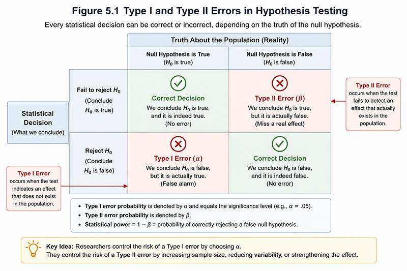
Throughout the remainder of this module, every statistical test involves balancing these two possibilities. The goal of hypothesis testing is therefore not to eliminate error completely—which is impossible—but to control the probability of making incorrect decisions to an acceptable level.
Because statistical decisions always involve some possibility of error, researchers specify in advance how much risk they are willing to accept before rejecting the null hypothesis. This predetermined probability is known as the significance level, represented by the Greek letter α (alpha).
The significance level represents the maximum probability of committing a Type I error that the researcher is prepared to tolerate. If the probability of obtaining the observed sample result under the null hypothesis is smaller than α, the observed evidence is considered sufficiently inconsistent with the null hypothesis to justify rejecting it.
In most scientific disciplines, three significance levels are commonly used:
| Significance Level | Interpretation |
|---|---|
| α = 0.10 | Allows a 10% risk of making a Type I error. Sometimes used for exploratory studies. |
| α = 0.05 | Allows a 5% risk of making a Type I error. This is the most commonly used significance level. |
| α = 0.01 | Allows only a 1% risk of making a Type I error. Often used when stronger evidence is required. |
Notice that smaller values of α require stronger evidence before the null hypothesis can be rejected. Consequently, using α = 0.01 makes it more difficult to declare statistical significance than using α = 0.05 or α = 0.10. Researchers therefore select α before analysing the data based on the importance of avoiding false positive conclusions within their field of study.
The significance level should never be chosen after examining the sample results. Changing α simply to obtain statistical significance undermines the objectivity of hypothesis testing and increases the likelihood of misleading conclusions. For this reason, good scientific practice requires the significance level to be specified before any statistical analysis is performed.
Throughout this module, you will discover that statistical significance depends not only on the observed data but also on the significance level chosen before the analysis begins. Understanding the role of α is therefore essential for interpreting every hypothesis test correctly.
One of the most misunderstood concepts in statistics is the p-value. Many learners memorise the rule "if p is less than 0.05, reject the null hypothesis" without understanding what the p-value actually represents. However, developing a correct interpretation of the p-value is essential because it forms the basis of statistical decision making.
The p-value is the probability of obtaining a sample result at least as extreme as the one observed, assuming that the null hypothesis is true. In other words, the p-value measures how surprising the observed data would be if the population actually behaved according to the null hypothesis.
Suppose a company claims that the average annual income of its customers is ₹70,000. After collecting a random sample, you observe a sample mean of ₹69,952. The question is not simply whether the sample mean differs from ₹70,000—every sample differs slightly because of random sampling variation. Instead, the important question becomes:
"If the true population mean really is ₹70,000, how likely is it that random sampling alone would produce a sample mean at least this different?"
The answer to this question is the p-value. A large p-value indicates that the observed sample is reasonably consistent with the null hypothesis because similar sample results would occur quite frequently by chance alone. Conversely, a very small p-value indicates that the observed sample would be highly unusual if the null hypothesis were true, providing evidence against the null hypothesis.
The p-value therefore measures the compatibility between the observed sample and the null hypothesis. Smaller p-values indicate greater incompatibility, while larger p-values indicate that the observed sample is reasonably plausible under the null hypothesis.
A common misconception is that the p-value represents the probability that the null hypothesis is correct. This interpretation is incorrect. The null hypothesis is either true or false—it does not have a probability attached to it. Instead, the p-value describes the probability of observing the data assuming that the null hypothesis is true.
Throughout this module, the LearnerBox Statistical Explorer calculates the p-value automatically while simultaneously displaying the rejection regions and observed test statistic on the sampling distribution. This allows you to see that the p-value is not simply another number—it represents the area of the sampling distribution beyond the observed test statistic under the null hypothesis.
While the p-value provides one method for making statistical decisions, hypothesis testing can also be understood visually using critical values and rejection regions. Both approaches always lead to the same statistical conclusion when applied correctly.
The sampling distribution predicted by the null hypothesis represents the range of sample statistics that would reasonably be expected through random sampling variation. Most sample statistics fall near the centre of this distribution, whereas extremely unusual values occur only within the tails.
Before analysing the data, the researcher selects a significance level (α), such as 0.05. This significance level determines the size of the rejection region. For a two-tailed hypothesis test with α = 0.05, the most extreme 5% of possible sample outcomes are designated as the rejection region, with 2.5% allocated to each tail of the distribution.
The boundary separating the non-rejection region from the rejection region is called the critical value. If the observed test statistic falls beyond the critical value, the sample is considered sufficiently unusual that the null hypothesis is rejected. Otherwise, the null hypothesis is not rejected.
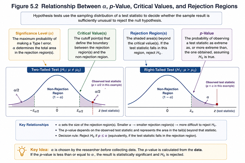
For example, when α = 0.05 and a two-tailed z-test is performed, the critical values are approximately ±1.96. Any observed z statistic larger than +1.96 or smaller than −1.96 falls within the rejection region. Values between −1.96 and +1.96 remain within the non-rejection region because they are considered reasonably plausible under the null hypothesis.
Although introductory statistics often presents the critical value approach and the p-value approach separately, they are simply two ways of expressing the same decision. If the observed test statistic falls inside the rejection region, the p-value will necessarily be smaller than α. Conversely, if the observed statistic remains inside the non-rejection region, the p-value will be larger than α.
The LearnerBox Statistical Explorer demonstrates this relationship visually. As you change the significance level or select one-tailed and two-tailed hypotheses, the rejection regions move automatically while the p-value is recalculated. This reinforces an important principle: statistical significance depends on both the observed data and the decision criterion selected before the analysis begins.
Up to this point, we have focused on controlling the probability of making a Type I error by selecting an appropriate significance level (α). However, researchers are also concerned with avoiding Type II errors, in which a genuine effect exists but the statistical test fails to detect it. The ability of a statistical test to correctly identify a real effect is known as its statistical power.
Statistical power is the probability that a hypothesis test will correctly reject the null hypothesis when the null hypothesis is actually false. A statistical test with high power is more likely to detect meaningful differences, relationships, or treatment effects when they truly exist within the population. Conversely, a test with low power may fail to detect genuine effects, resulting in incorrect conclusions that no evidence exists.
Several factors influence the statistical power of a hypothesis test, but the most important is the sample size. Larger samples provide more information about the population and reduce the amount of random sampling variation. As a result, genuine differences become easier to distinguish from random noise, increasing the probability of detecting real effects.
The magnitude of the true effect also influences statistical power. Large effects are generally easier to detect than very small effects because they produce larger differences between the observed sample and the null hypothesis. Finally, the chosen significance level affects power. Increasing α slightly increases statistical power because the rejection region becomes larger, although this simultaneously increases the probability of committing a Type I error.
Researchers therefore face an important balance. Selecting an extremely small significance level reduces the probability of false positive conclusions but may also reduce the ability to detect genuine effects. Collecting larger samples helps overcome this trade-off because it simultaneously improves the precision of estimates and increases statistical power without increasing the Type I error rate.
Throughout the LearnerBox Statistical Explorer, you will notice that changing the sample size immediately affects the standard error, confidence intervals, and hypothesis test results. This demonstrates one of the most important principles of inferential statistics: increasing the amount of information available generally leads to more precise estimation and more reliable statistical decisions.
You have now encountered the fundamental concepts that underpin every hypothesis test. We have learned how statistical hypotheses are formulated, why null and alternative hypotheses are required, how one-tailed and two-tailed tests differ, why statistical decisions are subject to Type I and Type II errors, how significance levels control the probability of false positive conclusions, how p-values measure evidence against the null hypothesis, and how rejection regions provide a visual decision rule for hypothesis testing.
These ideas form the conceptual foundation of inferential statistics. Regardless of whether a researcher performs a z-test, a t-test, an analysis of variance, a regression analysis, or a machine-learning significance test, the underlying statistical reasoning remains remarkably similar. The mathematical formulas may become more sophisticated, but the decision-making framework introduced in this chapter remains unchanged.
The next step is to apply these concepts to actual statistical procedures. We begin with the one-sample z-test, the simplest hypothesis test for comparing a sample mean with a known population value when the population standard deviation is available. Although z-tests are less common in practical research than t-tests, they provide an ideal introduction because they illustrate every component of statistical hypothesis testing in its simplest mathematical form.
Throughout the remainder of this module, the LearnerBox Statistical Explorer will accompany each statistical procedure. Rather than simply calculating answers, the Explorer allows you to visualise sampling distributions, modify hypotheses, change significance levels, compare confidence intervals, interpret statistical output, and generate APA-style results. By combining mathematical calculations with visual interpretation, you will develop a deeper understanding of why statistical decisions are made—not merely how they are calculated.
We now begin with the one-sample z-test, the foundation upon which all subsequent hypothesis tests are built.
The one-sample z-test is one of the simplest methods of statistical hypothesis testing. Its purpose is to determine whether the mean of a sample differs significantly from a known or hypothesised population mean. Although the z-test is introduced first in most statistics courses because of its mathematical simplicity, it is actually used less frequently in practical research than the t-test. Nevertheless, understanding the z-test provides an excellent foundation for learning every other hypothesis test presented later in this course.
The essential idea is straightforward. Suppose a company claims that the average annual income of its customers is ₹70,000. A researcher selects a random sample of customers and calculates the sample mean. Because every sample differs slightly through random sampling variation, the sample mean will almost never equal exactly ₹70,000. The question therefore becomes whether the observed difference is large enough that it is unlikely to have occurred by chance alone.
The z-test answers this question by comparing the observed sample mean with the hypothesised population mean while taking into account the amount of variability expected from random sampling. If the observed difference is much larger than would normally be expected, the null hypothesis is rejected. Otherwise, the observed difference is regarded as consistent with ordinary sampling variation.
One important characteristic distinguishes the z-test from other hypothesis tests. The z-test assumes that the population standard deviation (σ) is already known. This allows the amount of expected sampling variation to be calculated precisely using the standard error of the mean. Because the population standard deviation is rarely known in real-world research, the z-test is primarily used for teaching fundamental statistical concepts or in specialised applications where reliable population variability has been established through previous large-scale studies.
In this course, the LearnerBox Statistical Explorer allows you to investigate one-sample z-tests using a variety of variables from the customer purchase dataset. You can modify the hypothesised population mean, select one-tailed or two-tailed hypotheses, choose different significance levels, and immediately observe how these decisions affect the calculated z statistic, p-value, confidence interval, rejection regions, and statistical conclusion.
Throughout this section, remember that the z-test is not designed to measure how large the observed difference is in practical terms. Instead, it evaluates whether the observed evidence is sufficiently inconsistent with the null hypothesis to justify rejecting it. Practical importance will later be assessed using effect sizes and confidence intervals.
Like every statistical procedure, the one-sample z-test is based upon several assumptions. These assumptions ensure that the sampling distribution used to calculate probabilities accurately represents the behaviour of the sample statistic. Before performing any hypothesis test, researchers should always evaluate whether these assumptions are reasonably satisfied.
The first assumption is that the observations represent a random and independent sample from the population of interest. Random sampling ensures that every member of the population has an appropriate chance of selection, while independence means that one observation does not influence another. Violations of independence can substantially affect the validity of statistical conclusions.
The second assumption is that the variable being analysed is measured on an interval or ratio scale. Since the z-test compares population means, the data should be numerical rather than purely categorical.
The third assumption concerns the shape of the population distribution. Ideally, the population should be approximately normally distributed. However, because of the Central Limit Theorem introduced in Module 4, the sampling distribution of the sample mean becomes approximately normal whenever the sample size is sufficiently large, even if the original population distribution is moderately skewed. Consequently, the normality assumption becomes less restrictive for large samples.
The fourth—and most important—assumption is that the population standard deviation (σ) is known. This assumption distinguishes the z-test from the t-test. When σ is unknown, which is the situation encountered in most practical research, the sampling variability must instead be estimated from the sample itself, leading naturally to Student's t-distribution. This important difference will be explored later in this module.
Fortunately, the LearnerBox Statistical Explorer makes this distinction immediately visible. When performing confidence intervals or hypothesis tests, simply switching between Known Population Standard Deviation and Unknown Population Standard Deviation automatically changes the underlying statistical method from the z distribution to the t distribution. This allows you to observe how the mathematical assumptions influence the statistical procedure while the sample data remain unchanged.
In the next sections, we examine why knowledge of the population standard deviation is so important and how it leads directly to the concept of the standard error of the mean, one of the most fundamental quantities in inferential statistics.
One characteristic distinguishes the one-sample z-test from nearly every other hypothesis test introduced later in this course: the population standard deviation (σ) is assumed to be known. Although this assumption may appear minor, it fundamentally determines how uncertainty is measured and why the z-test uses the standard normal distribution.
Recall from Module 4 that individual observations within a population naturally vary. This variability is measured by the population standard deviation, σ. When σ is known, we can determine how much variability should be expected in the distribution of sample means. This quantity is known as the standard error of the mean.
The standard error measures the average amount by which sample means are expected to differ from the true population mean because of random sampling alone. Unlike the population standard deviation, which describes the variability of individual observations, the standard error describes the variability of sample means.
The standard error of the mean is calculated using the following formula:
\[ SE = \frac{\sigma}{\sqrt{n}} \]where:
This equation contains one of the most important ideas in inferential statistics. As the sample size increases, the denominator becomes larger, causing the standard error to decrease. In other words, larger samples produce more stable and more precise estimates of the population mean because random sampling variation becomes smaller.
For example, suppose the population standard deviation is known to be σ = 10.
| Sample Size (n) | Standard Error |
|---|---|
| 25 | \(\frac{10}{\sqrt{25}}=2.00\) |
| 100 | \(\frac{10}{\sqrt{100}}=1.00\) |
| 400 | \(\frac{10}{\sqrt{400}}=0.50\) |
Notice that increasing the sample size by a factor of four halves the standard error. This relationship explains why researchers often prefer larger samples—they reduce random sampling variability and produce more precise estimates of the population mean.
Within the LearnerBox Statistical Explorer, the standard error is calculated automatically whenever a known population standard deviation is entered. As you increase the sample size, notice how the standard error decreases, the confidence interval becomes narrower, and the statistical conclusions become more precise. This illustrates one of the central ideas of inferential statistics: more information generally leads to more reliable decisions.
Now that we understand the concept of the standard error, we can derive the z statistic itself. The goal of every hypothesis test is to determine whether the observed sample mean differs from the hypothesised population mean by more than would reasonably be expected through random sampling variation alone.
The first step is to calculate the observed difference:
\[ \text{Observed Difference} = \bar{x} - \mu_0 \]where:
By itself, however, the observed difference tells us very little. A difference of two units may be extremely important in one situation yet completely negligible in another. The interpretation depends upon the amount of variability expected through random sampling.
To account for this variability, we divide the observed difference by the standard error. This converts the observed difference into a standardised value measured in units of standard errors.
\[ z = \frac{\bar{x} - \mu_0}{SE} \]Substituting the expression for the standard error gives the familiar one-sample z-test formula:
\[ z=\frac{\bar{x}-\mu_0}{\sigma/\sqrt{n}} \]This formula compares two quantities:
If the observed difference is small relative to the standard error, the resulting z statistic will be close to zero, indicating that the sample is consistent with the null hypothesis. If the observed difference is several standard errors away from the hypothesised mean, the z statistic becomes large in magnitude, suggesting that the observed sample would be unlikely if the null hypothesis were true.
An important feature of the z statistic is that it has no units. Whether annual income is measured in rupees, customer satisfaction on a ten-point scale, or response time in minutes, the z statistic always represents the number of standard errors separating the observed sample mean from the hypothesised population mean.
The LearnerBox Statistical Explorer performs this calculation automatically. As you modify the hypothesised population mean, sample size, or known population standard deviation, observe how the standard error changes and how this affects the calculated z statistic. This dynamic relationship is much easier to appreciate visually than by studying the formula alone.
In the next section, we will use this formula to calculate the z statistic step by step before learning how statistical decisions are made using critical values and p-values.
Once the standard error has been calculated, computing the z statistic is straightforward. The z statistic measures how many standard errors separate the observed sample mean from the hypothesised population mean specified by the null hypothesis.
\[ z=\frac{\bar{x}-\mu_0}{\sigma/\sqrt{n}} \]The calculation follows a series of logical steps:
Suppose a company claims that its customers spend an average of ₹70,000 annually. A random sample of 100 customers produces a sample mean of ₹69,952. Assume that previous large-scale studies have established the population standard deviation to be σ = ₹10.
The first step is to calculate the standard error:
\[ SE=\frac{10}{\sqrt{100}}=\frac{10}{10}=1.00 \]Next, calculate the observed difference:
\[ \bar{x}-\mu_0=69,952-70,000=-48 \]Finally, divide this difference by the standard error:
\[ z=\frac{-48}{1.00}=-48.00 \]The resulting z statistic indicates that the observed sample mean lies 48 standard errors below the hypothesised population mean. Such an extreme value would be extraordinarily unlikely if the null hypothesis were true.
Notice that the z statistic is always interpreted relative to zero. A value of zero indicates perfect agreement between the sample mean and the hypothesised population mean. Positive z values indicate that the sample mean exceeds the hypothesised value, whereas negative z values indicate that the sample mean is smaller than the hypothesised value.
Within the LearnerBox Statistical Explorer, the z statistic is calculated automatically as soon as the hypothesised mean or population standard deviation is changed. Rather than memorising the calculation, learners can concentrate on understanding how each component influences the final statistical decision.
Calculating the z statistic is only the first stage of hypothesis testing. The next task is to determine whether the observed value provides sufficient evidence to reject the null hypothesis. Two equivalent approaches may be used: the critical value approach and the p-value approach. Both methods always lead to the same statistical conclusion.
When using the critical value approach, the calculated z statistic is compared with one or more critical values determined by the significance level (α) and the form of the alternative hypothesis.
For example, if α = 0.05:
If the calculated z statistic falls beyond the appropriate critical value, the null hypothesis is rejected. Otherwise, the null hypothesis is not rejected.
The p-value approach compares the probability of observing the calculated z statistic with the chosen significance level.
Because both approaches are mathematically equivalent, researchers generally report the p-value while many textbooks continue to teach the critical value approach because it provides valuable insight into how hypothesis testing operates.
After making the statistical decision, the results should always be interpreted in the context of the research question rather than simply reporting numerical values. A complete interpretation usually includes four components:
For example, suppose a two-tailed z-test produced the following results:
Because the p-value is much smaller than the chosen significance level, the null hypothesis is rejected. The evidence suggests that the population mean annual income differs significantly from ₹70,000.
Notice that statistical significance does not automatically imply practical importance. A very small difference may become statistically significant if the sample size is sufficiently large. For this reason, researchers should interpret hypothesis tests alongside confidence intervals and effect-size measures whenever possible.
We are now ready to perform complete hypothesis tests using real data from the LearnerBox customer purchase dataset. The worked examples that follow will demonstrate each stage of the hypothesis-testing process, from stating the hypotheses to reporting the results in APA style.
Before completing our study of the one-sample z-test, it is useful to return briefly to one of the central ideas introduced in Module 4: the confidence interval. At first glance, confidence intervals and hypothesis tests appear to be different statistical procedures. One estimates an unknown population parameter, while the other evaluates a research hypothesis. In reality, they are two different ways of answering the same inferential question.
Suppose a researcher constructs a 95% confidence interval for the population mean. If the hypothesised population mean specified by the null hypothesis lies inside this interval, the observed sample is considered reasonably consistent with the null hypothesis, and the null hypothesis is not rejected at α = .05. Conversely, if the hypothesised population mean lies outside the confidence interval, the observed sample provides sufficient evidence to reject the null hypothesis.
This relationship exists because both procedures are based upon exactly the same sampling distribution and significance level. The confidence interval estimates the range of plausible population values, while the hypothesis test asks whether one particular value remains plausible.
The LearnerBox Statistical Explorer displays both the confidence interval and the hypothesis test simultaneously. As you experiment with different significance levels and hypothesised means, notice that both approaches always lead to the same statistical conclusion.
Research Question
Does the mean annual income of customers differ from ₹70,000?
Data
Step 1 — State the hypotheses
\[ \bar{x} - \mu_0 = 69{,}952 - 70{,}000 = -48 \] \[ H_1: \mu \neq 70{,}000 \]Step 2 — Calculate the standard error
\[ SE=\frac{10}{\sqrt{100}}=1.00 \]Step 3 — Calculate the z statistic
\[ z = \frac{69{,}952 - 70{,}000}{1.00} = -48.00 \]Step 4 — Make the statistical decision
For a two-tailed test at α = .05, the critical values are ±1.96. Since z = −48.00 falls well beyond −1.96, the null hypothesis is rejected.
Step 5 — Interpret the result
The sample mean lies 48 standard errors below the hypothesised population mean. Such an extreme result would be extraordinarily unlikely if the true population mean were ₹70,000.
The data remain exactly the same as Worked Example 5.1. Only the research question changes.
Research Question
Is the mean annual income greater than ₹70,000?
\[ H_0: \mu \leq 70{,}000 \] \[ H_1: \mu > 70{,}000 \]The calculated z statistic is still:
\[ z = -48.00 \]However, because the research question is now right-tailed, only the upper tail of the sampling distribution forms the rejection region. The critical value becomes +1.645.
Since the observed z statistic lies far to the left of the distribution, it provides no evidence that the population mean exceeds ₹70,000.
The p-value is therefore much larger than .05, and the null hypothesis is not rejected.
When students first learn inferential statistics, confidence intervals and hypothesis tests often appear to be separate statistical techniques. Confidence intervals seem to estimate population parameters, whereas hypothesis tests appear to answer research questions. Although these interpretations are correct, they overlook a much deeper connection. Both procedures are built upon exactly the same probability model and therefore communicate the same statistical evidence in different forms.
A confidence interval identifies a range of population values that are consistent with the observed sample. A hypothesis test, on the other hand, evaluates whether one specific population value remains consistent with the observed sample. The only difference lies in presentation. Confidence intervals answer the question, "Which population values are plausible?" Hypothesis tests answer the question, "Is this particular population value still plausible?"
Suppose a researcher constructs a 95% confidence interval for the population mean annual income. If the interval extends from ₹69,950 to ₹69,954, then every value inside this interval is considered reasonably consistent with the observed sample. If the hypothesised value of ₹70,000 lies outside this interval, the corresponding hypothesis test will reject the null hypothesis at the 5% significance level.
This relationship is not a coincidence. Both procedures rely upon the same standard error, the same sampling distribution, and the same confidence level. Consequently, whenever the confidence interval excludes the hypothesised population value, the corresponding hypothesis test will reject the null hypothesis. Likewise, whenever the hypothesised value lies within the confidence interval, the null hypothesis will not be rejected.
The width of every confidence interval depends upon a quantity known as the margin of error. The margin of error represents the maximum distance between the sample estimate and either end of the confidence interval. In other words, it measures the uncertainty associated with estimating the population parameter from a sample.
For a confidence interval based on the normal distribution, the margin of error is calculated by multiplying the critical value by the standard error:
\[ \text{Margin of Error} = \text{Critical Value} \times \text{Standard Error} \]For example, suppose a researcher constructs a 95% confidence interval using a standard error of 1.581. Since the critical z value for a 95% confidence interval is 1.96, the margin of error is: \(1.96 \times 1.581 = 3.099\)
The confidence interval is therefore calculated as: \(72.000 \pm 3.099\)
resulting in a confidence interval extending from 68.901 to 75.099.
Several factors influence the margin of error. Larger samples reduce the standard error, leading to narrower confidence intervals. Increasing the confidence level has the opposite effect because larger critical values produce wider intervals. Researchers therefore balance precision against confidence when designing statistical studies.
The confidence level specifies how often the interval construction procedure would successfully capture the true population parameter if the sampling process were repeated many times under identical conditions. A 95% confidence level therefore means that approximately 95% of confidence intervals constructed using this method would contain the true population parameter, while approximately 5% would not.
This interpretation is frequently misunderstood. The confidence level does not mean that there is a 95% probability that the true population mean lies inside one particular confidence interval. Once the interval has been calculated, the population parameter either lies within it or it does not. Instead, the 95% refers to the long-run performance of the interval estimation procedure.
Suppose the null hypothesis states that the population mean annual income equals ₹70,000. After constructing a 95% confidence interval, the researcher discovers that ₹70,000 lies comfortably inside the interval.
In this situation, the observed sample is considered reasonably consistent with the null hypothesis because the hypothesised value remains one of the plausible population values suggested by the data. Consequently, there is insufficient statistical evidence to reject the null hypothesis at the 5% significance level.
Notice that this does not prove the null hypothesis to be true. It simply indicates that the available sample evidence does not provide sufficient justification for rejecting it. A different sample might produce a narrower confidence interval or a different estimate that leads to another conclusion.
Now consider the opposite situation. Suppose the hypothesised population mean is ₹70,000, but the 95% confidence interval extends only from ₹69,950 to ₹69,954. Because ₹70,000 lies outside the interval, the hypothesised value is no longer considered consistent with the observed sample.
This immediately leads to the same conclusion that would have been reached using the corresponding hypothesis test. The null hypothesis is rejected because the observed evidence suggests that the hypothesised population value is implausible given the sample data.
This simple visual interpretation explains why confidence intervals are widely preferred in many scientific publications. Rather than reporting only whether a result is statistically significant, confidence intervals also indicate the magnitude and precision of the estimated effect, providing substantially more information than a single p-value.
Research Question
Using the Annual Income variable, estimate the population mean annual income and determine whether the hypothesised value of ₹70,000 remains plausible.
Results from the LearnerBox Statistical Explorer
Interpretation
The 95% confidence interval extends from 68.901 to 75.099. Because the hypothesised population mean of 70.000 lies inside this interval, the observed sample remains consistent with the null hypothesis. Therefore, the corresponding two-tailed hypothesis test at α = .05 would fail to reject the null hypothesis.
Rather than focusing on the p-value, notice how the confidence interval immediately communicates both the estimated population mean and the uncertainty associated with that estimate. Any population value inside the interval is considered reasonably plausible given the observed sample.
After learning the one-sample z-test, many students assume that it is the standard procedure used by researchers. Surprisingly, the opposite is true. Although the z-test provides an excellent introduction to hypothesis testing, it is used relatively rarely in practical research because one of its most important assumptions is almost never satisfied.
Recall that the z-test requires the population standard deviation (σ) to be known. In real investigations, researchers rarely have access to the entire population and therefore cannot calculate the true population standard deviation. Instead, they collect a sample and estimate the population variability using the sample standard deviation (s).
Replacing the unknown population standard deviation with the sample standard deviation introduces additional uncertainty into the analysis. The sample standard deviation is itself an estimate and therefore varies from one random sample to another. Consequently, the sampling distribution of the test statistic is no longer described perfectly by the standard normal distribution.
This problem was solved by the English statistician William Sealy Gosset, who developed a new probability distribution while working for the Guinness Brewery in Dublin. Because his employer prohibited employees from publishing research under their own names, Gosset published under the pseudonym "Student". The resulting probability model became known as Student's t-distribution, and the associated hypothesis test became the t-test.
Today, nearly all hypothesis tests comparing sample means use one of the various forms of the t-test rather than the z-test. Modern statistical software automatically performs t-tests because they remain valid whether the population standard deviation is known or unknown. As the sample size becomes large, the t-distribution gradually approaches the standard normal distribution, making the difference between the two procedures negligible.
The z-test therefore remains extremely valuable—not because it is used frequently in research, but because it introduces the fundamental logic of hypothesis testing. Once that logic has been understood, replacing the z-distribution with the t-distribution becomes a natural extension rather than an entirely new statistical procedure.
The Student's t-distribution is a probability distribution specifically designed for situations in which the population standard deviation is unknown. Like the standard normal distribution, it is continuous, symmetric, and centred on zero. However, it possesses an important additional characteristic: its tails are slightly thicker than those of the normal distribution.
These heavier tails reflect the additional uncertainty introduced when the population standard deviation must be estimated from the sample rather than known exactly. Because the estimate of variability changes from one sample to another, extreme sample means occur slightly more often than would be predicted by the standard normal distribution. The t-distribution therefore assigns greater probability to values farther from the centre.
An interesting feature of the t-distribution is that it does not represent a single curve. Instead, it represents an entire family of distributions. Each member of this family is determined by a quantity known as the degrees of freedom. Smaller degrees of freedom produce heavier tails because the estimate of variability is based on relatively little information. As the degrees of freedom increase, the estimate of variability becomes more reliable and the t-distribution gradually approaches the standard normal distribution.
This behaviour explains why large-sample t-tests produce results that are almost identical to corresponding z-tests. When the sample size becomes sufficiently large, the additional uncertainty associated with estimating the population standard deviation becomes very small, and the distinction between the two distributions largely disappears.
The LearnerBox Statistical Explorer demonstrates this difference automatically. When the population standard deviation is specified as known, confidence intervals and hypothesis tests use the z-distribution. When the population standard deviation is unknown, the Explorer immediately switches to the appropriate t-distribution, adjusts the critical values, and reports the corresponding degrees of freedom.
One of the most distinctive features of the t-distribution is that its exact shape depends upon the degrees of freedom (df). Degrees of freedom measure the amount of independent information available for estimating population variability after certain quantities have already been estimated from the sample.
Although the term may initially sound abstract, the underlying idea is surprisingly simple. Suppose a sample contains five observations with a fixed mean. Once four observations have been chosen, the fifth observation can no longer vary freely because its value is completely determined by the requirement that the sample must retain the specified mean. In effect, only four observations remain free to vary independently. The sample therefore possesses four degrees of freedom.
For the one-sample t-test, the degrees of freedom are calculated using the simple relationship: \(df = n - 1\) where n represents the sample size. Thus, a sample containing 40 observations has 39 degrees of freedom, while a sample containing 100 observations has 99 degrees of freedom.
Degrees of freedom determine which member of the t-distribution family should be used. Smaller samples produce fewer degrees of freedom, resulting in heavier tails and larger critical values. Larger samples produce more degrees of freedom, causing the t-distribution to become progressively closer to the standard normal distribution.
Although the normal distribution and the Student's t-distribution appear visually similar, they differ in one important respect. The t-distribution allocates slightly more probability to values farther from the centre of the distribution. This characteristic produces larger critical values and therefore slightly wider confidence intervals and more conservative hypothesis tests when sample sizes are small.
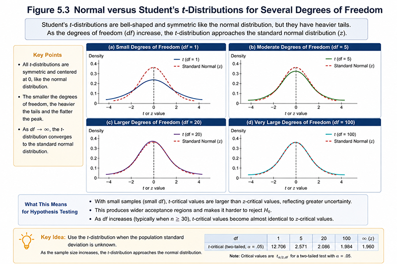
As the sample size increases, the estimate of the population standard deviation becomes increasingly stable. Consequently, the additional uncertainty accounted for by the t-distribution gradually disappears, and the t-distribution becomes almost indistinguishable from the standard normal distribution.
For this reason, large-sample t-tests and z-tests often produce almost identical numerical results. Nevertheless, researchers generally continue to use the t-test because it remains valid regardless of whether the population standard deviation is known, whereas the z-test requires an assumption that is rarely satisfied in practice.
Having established why the t-distribution is required, we can now examine the assumptions that underlie all forms of the t-test and learn how these assumptions should be assessed before statistical analyses are performed.
Before performing any statistical hypothesis test, researchers should verify that the underlying assumptions of the analysis are reasonably satisfied. Every statistical procedure is based upon a mathematical model describing how the data are expected to behave. When these assumptions are seriously violated, the resulting p-values, confidence intervals, and statistical conclusions may no longer be reliable.
Fortunately, the t-test is remarkably robust. Moderate departures from some assumptions have relatively little influence on the validity of the analysis, particularly when sample sizes are reasonably large. Nevertheless, good statistical practice requires that assumptions be assessed before interpreting the results.
The dependent variable analysed by a t-test should be measured on an interval or ratio scale. Variables such as annual income, customer age, response time, purchase amount, credit score, or customer satisfaction are appropriate because numerical differences between observations are meaningful.
Categorical variables such as gender, loyalty tier, or location type cannot themselves be analysed using a t-test because they do not represent continuous measurements. However, they may be used as grouping variables in an independent-samples t-test.
This assumption is assessed simply by examining the type of variable being analysed. No statistical test is required.
Independence means that each observation contributes unique information to the analysis. The value recorded for one participant should not influence the value recorded for another participant.
This assumption is generally satisfied through appropriate study design rather than statistical testing. Random sampling and independent selection of participants usually ensure independence. Violations may occur when repeated observations are incorrectly analysed as independent measurements or when participants influence one another during data collection.
For paired-samples t-tests, independence is required between pairs, although the two observations within each pair are intentionally related.
The t-test assumes that the variable being analysed—or, in the case of a paired-samples t-test, the difference scores—is approximately normally distributed within the population. Fortunately, because of the Central Limit Theorem introduced in Module 4, moderate departures from normality become less important as the sample size increases.
Several methods are commonly used to assess this assumption:
For both the Shapiro–Wilk and Kolmogorov–Smirnov tests, the null hypothesis states that the data follow a normal distribution. Therefore:
Researchers should remember that formal normality tests become extremely sensitive when sample sizes are large. Even trivial departures from normality may produce statistically significant results. Consequently, visual methods such as histograms and Q–Q plots should always be interpreted alongside formal statistical tests.
For the independent-samples t-test, the variability of the dependent variable should be reasonably similar across the groups being compared. This assumption is known as homogeneity of variance.
Traditionally, this assumption has been assessed using Levene's test. The null hypothesis of Levene's test states that the group variances are equal.
Historically, researchers selected the classical Student's t-test when Levene's test was non-significant and switched to Welch's t-test only when unequal variances were detected. However, this approach has changed considerably over the past decade.
Although checking assumptions is an essential part of statistical analysis, researchers should avoid treating them as rigid pass–fail rules. The t-test is well known for its robustness, particularly when sample sizes are moderate or large. Small departures from normality rarely invalidate the analysis, and modern methods such as Welch's t-test effectively address unequal variances without requiring separate preliminary decisions.
The most serious violations typically involve problems with study design, such as lack of independence between observations. These issues cannot be corrected statistically after the data have been collected, emphasising the importance of careful experimental design before any analysis begins.
The one-sample t-test is used to determine whether the mean of a sample differs significantly from a known or hypothesised population mean when the population standard deviation is unknown. Because the population standard deviation is rarely available in practical research, the one-sample t-test has become one of the most widely used procedures in inferential statistics.
Conceptually, the one-sample t-test asks exactly the same question as the one-sample z-test:
"Is the observed sample mean sufficiently different from the hypothesised population mean that the difference is unlikely to have occurred through random sampling variation alone?"
The difference lies not in the research question but in the information available. Whereas the z-test assumes knowledge of the true population standard deviation (σ), the one-sample t-test estimates population variability using the sample standard deviation (s). This additional uncertainty is accommodated by the Student's t-distribution introduced in the previous section.
The one-sample t-test is particularly useful when comparing a sample mean with a benchmark or target value. For example, a bank may wish to determine whether the average credit score of its customers differs from an industry benchmark of 650. Similarly, a hospital may compare the average patient waiting time with a recommended national standard, or an educational institution may compare students' examination scores with a desired performance level.
Throughout this section, we shall use the Credit Score variable from the LearnerBox customer purchase dataset to illustrate the one-sample t-test. The LearnerBox Statistical Explorer automatically calculates the sample standard deviation, standard error, t statistic, degrees of freedom, p-value, confidence interval, and effect size, allowing you to concentrate on interpreting the statistical results rather than performing repetitive calculations.
The mathematical reasoning behind the one-sample t-test closely resembles that of the one-sample z-test. Once again, the objective is to compare the observed sample mean with the hypothesised population mean while accounting for the amount of variation expected through random sampling.
The observed difference remains: \(\bar{x} - \mu_0\)
However, because the population standard deviation is unknown, the standard error must now be estimated using the sample standard deviation: \( SE=\frac{s}{\sqrt{n}}\)
Replacing σ with s leads directly to the one-sample t statistic: \[SE = \frac{s}{\sqrt{n}}\]
\[ t=\frac{\bar{x}-\mu_0}{s/\sqrt{n}} \]Notice how remarkably similar this expression is to the z-test formula. In fact, the only mathematical difference is the replacement of the unknown population standard deviation by the sample standard deviation. Nevertheless, this apparently small change has important consequences because the sample standard deviation itself varies from one random sample to another. Consequently, the resulting test statistic follows Student's t-distribution rather than the standard normal distribution.
The t statistic, like the z statistic, measures the number of estimated standard errors separating the observed sample mean from the hypothesised population mean. Large positive or negative values indicate that the observed sample is unlikely to have arisen if the null hypothesis were true.
Within the LearnerBox Statistical Explorer, this transition is almost effortless. Selecting Unknown Population Standard Deviation automatically replaces the z statistic with the t statistic, recalculates the standard error using the sample standard deviation, updates the critical values, and reports the appropriate degrees of freedom.
Unlike the z-test, the one-sample t-test requires the researcher to specify the appropriate degrees of freedom (df). As discussed earlier, the degrees of freedom determine which member of the Student's t-distribution family should be used when calculating probabilities and critical values.
For the one-sample t-test, the degrees of freedom are calculated as: \(df = n - 1\)
This simple relationship arises because one parameter—the sample mean—must first be estimated from the data. Once the sample mean has been calculated, only n − 1 observations remain free to vary independently.
For example, if a study contains 100 observations:
\(df = 100 - 1 = 99\)The hypothesis test therefore uses the t-distribution corresponding to 99 degrees of freedom. Because this represents a relatively large sample, the resulting t-distribution is already very close to the standard normal distribution.
As the sample size decreases, the degrees of freedom also decrease, producing heavier tails and larger critical values. This makes the hypothesis test slightly more conservative because greater evidence is required before rejecting the null hypothesis. Conversely, as the sample size increases, the t-distribution gradually converges towards the normal distribution, and the distinction between the two procedures becomes negligible.
The LearnerBox Statistical Explorer calculates the degrees of freedom automatically and displays the corresponding t-distribution used for the analysis. As you experiment with different sample sizes, notice how the reported degrees of freedom change and how the critical values gradually move closer to those of the standard normal distribution.
The one-sample t-test begins by defining a null hypothesis and an alternative hypothesis. As with the z-test, these hypotheses must be stated before examining the statistical results because the form of the alternative hypothesis determines whether the test is two-tailed, right-tailed, or left-tailed.
The null hypothesis (H₀) states that the population mean is equal to the hypothesised value. The alternative hypothesis (H₁) describes the difference or direction proposed by the research question.
For a two-tailed one-sample t-test:
\[ H_0: \mu = \mu_0 \] \[ H_1: \mu \neq \mu_0 \]A two-tailed test is appropriate when the research question asks whether the population mean differs from the hypothesised value without predicting a particular direction.
For a right-tailed test:
\[ H_0: \mu \leq \mu_0 \] \[ H_1: \mu > \mu_0 \] H₀: μ ≤ μ₀This form is used when the research question specifically predicts that the population mean is greater than the hypothesised value.
For a left-tailed test:
\[ H_0: \mu \geq \mu_0 \] \[ H_1: \mu < \mu_0 \]A left-tailed test is appropriate when the research question predicts that the population mean is smaller than the hypothesised value.
After stating the hypotheses, the researcher selects the significance level (α). In many studies, α = .05 is used, although α = .01 may be selected when stronger evidence is required and α = .10 may sometimes be used in exploratory research.
The LearnerBox Statistical Explorer allows all three hypothesis directions and several significance levels to be examined using the same dataset. This makes it possible to observe how the research hypothesis and decision criterion influence the rejection region and statistical conclusion while the underlying sample data remain unchanged.
A complete interpretation of a one-sample t-test involves considerably more than determining whether the p-value is statistically significant. Good statistical analysis follows a sequence of reasoning that begins with the research question, evaluates the assumptions of the test, examines the test statistic and p-value, considers the magnitude of the effect, and finally communicates the conclusion in the context of the study.
The t statistic indicates how many estimated standard errors separate the sample mean from the hypothesised population mean. A positive t statistic indicates that the sample mean lies above the hypothesised value, whereas a negative t statistic indicates that the sample mean lies below it. The larger the absolute value of t, the greater the discrepancy between the observed sample and the null hypothesis relative to sampling variability.
The p-value then indicates how unusual a result at least this extreme would be if the null hypothesis were true. If p ≤ α, the null hypothesis is rejected. If p > α, the null hypothesis is not rejected.
However, statistical significance does not describe the magnitude of the observed difference. For this reason, hypothesis tests should be accompanied by an effect-size measure. For a one-sample t-test, a commonly reported effect size is Cohen's d:
\[ d=\frac{\bar{x}-\mu_0}{s} \]Cohen's d expresses the difference between the sample mean and the hypothesised population mean in units of the sample standard deviation. The sign indicates the direction of the difference, while the absolute magnitude indicates the size of the effect.
| Absolute Cohen's d | Conventional Interpretation |
|---|---|
| Approximately 0.20 | Small effect |
| Approximately 0.50 | Medium effect |
| Approximately 0.80 | Large effect |
These values should be treated as general guidelines rather than rigid boundaries. The practical importance of an effect always depends upon the research context. A statistically small effect may be highly important in medicine, public policy, finance, or large-scale educational interventions.
The following worked examples apply this complete workflow to the Credit Score variable in the LearnerBox customer purchase dataset.
Research Question
Does the mean credit score of customers differ from the hypothesised benchmark of 650?
Step 1 — Identify the test
The analysis compares the mean of one sample with a hypothesised population value. The population standard deviation is unknown. Therefore, a one-sample t-test is appropriate.
Step 2 — Check the assumptions
Credit Score is a continuous numerical variable, satisfying the measurement-level requirement. Each customer contributes one credit score to the dataset, so the observations are treated as independent.
The normality of Credit Score is assessed using the Shapiro–Wilk test: \[ W = 0.934, p < 0.00001 \] Since the p value is less than 0.05, we may not assume normal distribution. However, because the sample contains 150 observations, the one-sample t-test is reasonably robust to moderate departures from normality. The normality result should therefore be considered alongside the distribution of the data rather than treated as a rigid pass–fail rule.
Step 3 — State the hypotheses
\[ H_0: \mu = 650 \] \[ H_1: \mu \neq 650 \]Because the research question asks whether the mean credit score differs from 650 without specifying a direction, a two-tailed test is used.
Step 4 — Select the significance level: \( \alpha = .05 \)
Step 5 — Examine the sample statistics
The observed mean difference is: \( 617.180 - 650 = -32.820 \)
The sample mean is therefore 32.820 points below the hypothesised population mean.
Step 6 — Calculate the standard error
\[ SE=\frac{86.593}{\sqrt{150}}=7.070 \]Step 7 — Calculate the t statistic
\[ t=\frac{617.180-650}{86.593/\sqrt{150}}, t=-4.642 \]With 150 observations: \(df = 150 - 1 = 149\)
The sample mean lies approximately 4.64 estimated standard errors below the hypothesised population mean.
Step 8 — Interpret the p-value and make the statistical decision
The LearnerBox Statistical Explorer reports p < .0001. Because the p-value is smaller than α = .05, the null hypothesis is rejected.
There is sufficient statistical evidence to conclude that the population mean credit score differs from 650.
Step 9 — Examine the confidence interval
The 95% confidence interval for the population mean extends from 603.209 to 631.151. The hypothesised value of 650 lies outside this interval, leading to the same conclusion as the hypothesis test.
Step 10 — Calculate and interpret Cohen's d
\[ d=\frac{617.180-650}{86.593} \] \[ d=-0.379 \]The negative sign indicates that the sample mean lies below the hypothesised value. The absolute magnitude, |d| = 0.379, is conventionally interpreted as a small effect approaching medium magnitude. Thus, although the difference is highly statistically significant, its magnitude should be interpreted separately from the p-value.
Step 11 — State the conclusion in plain language
The analysis provides strong statistical evidence that the mean credit score of customers differs from the benchmark of 650. The observed customer mean is lower than the benchmark by approximately 20.62 credit-score points, with an effect of small-to-moderate magnitude.
Research Question
Is the mean credit score of customers lower than 650?
Step 1 — Identify the test
One sample mean is being compared with a hypothesised population value, and the population standard deviation is unknown. A one-sample t-test is therefore appropriate.
Step 2 — Check the assumptions
Credit Score is a continuous numerical variable, and each customer contributes one independent observation. The Shapiro–Wilk test of normality produces:
\[ W = 0.934, p < 0.00001 \]Step 3 — State the hypotheses
\[ H_0: \mu \geq 650 \] \[ H_1: \mu < 650 \]The research question specifically predicts that the mean credit score is lower than 650. A left-tailed hypothesis test is therefore appropriate.
Step 4 — Select the significance level: \( \alpha = .05 \)
Step 5 — Examine the test statistic
The sample statistics remain unchanged:
The calculated test statistic is:\(t = -4.642 \)
with 149 degrees of freedom.
The negative t statistic indicates that the sample mean lies below the hypothesised population mean. Importantly, this direction is consistent with the left-tailed alternative hypothesis.
Step 6 — Interpret the p-value and make the statistical decision
For the left-tailed test, the observed t statistic lies within the lower rejection region. The corresponding one-tailed p-value is less than .001.
Because p < .001 is smaller than α = .05, the null hypothesis is rejected.
There is sufficient statistical evidence to conclude that the population mean credit score is lower than 650.
Step 7 — Interpret the effect size
Cohen's d remains: \( d = -0.38 \)
Changing from a two-tailed to a left-tailed hypothesis does not change the observed mean difference, sample standard deviation, or effect size. The effect remains small-to-moderate in magnitude and is directed below the hypothesised benchmark.
Step 8 — State the conclusion in plain language
The customer data provide strong evidence that the population mean credit score is below 650. The observed mean is approximately 20.62 points below the hypothesised benchmark, and the magnitude of this difference is small to moderate.
The independent-samples t-test, also known as the two-sample t-test, is used to determine whether the population means of two independent groups differ significantly. Unlike the one-sample t-test, which compares one sample mean with a hypothesised value, the independent-samples t-test compares two sample means with one another.
For example, a researcher may wish to compare average purchase amounts between VIP and Regular customers, mean customer satisfaction between mobile-app users and non-users, or average age between customers living in urban and rural locations. In each case, the outcome variable is continuous, while a categorical grouping variable divides the observations into two distinct groups.
The central question is:
Does the observed difference between the two sample means provide sufficient evidence that the corresponding population means are genuinely different, or could the difference reasonably have arisen through random sampling variation?
Because two samples are involved, the analysis must account for the variability within each group as well as the number of observations in each group. A difference of five units may be persuasive when both groups have very little variability, but the same difference may provide weak evidence when the observations are widely dispersed.
The independent-samples t-test therefore standardises the observed difference between the group means using the estimated standard error of that difference. The resulting t statistic indicates how many standard errors separate the two sample means under the assumption that the null hypothesis is true.
The null hypothesis normally states that the two population means are equal:
\[ H_0:\mu_1=\mu_2 \]This may also be written as:
\[ H_0:\mu_1-\mu_2=0 \]For a two-tailed test, the alternative hypothesis states:
\[ H_1:\mu_1\neq\mu_2 \]Directional alternatives may also be used when the research question predicts that one population mean is greater than or less than the other. As always, the direction must be specified before examining the sample results.
In the worked examples that follow, the LearnerBox Statistical Explorer will be used to compare Age between Urban and Rural customers and Purchase Amount between VIP and Regular customers. These examples will also demonstrate how assumption testing, Welch's t-test, confidence intervals, effect size, and APA reporting form part of one complete analytical workflow.
The defining feature of the independent-samples t-test is that the two groups must be independent. This means that each observation belongs to one group only and that the value recorded for one participant does not determine or influence the value recorded for a participant in the other group.
For example, suppose customers are classified according to Location Type:
Each customer belongs to only one location category. The age of an Urban customer is not paired with the age of a particular Rural customer, and there is no requirement that the two groups contain the same number of observations. These are therefore independent groups.
The same reasoning applies when comparing VIP and Regular customers. A customer cannot belong to both loyalty tiers simultaneously, and the purchase amount recorded for one VIP customer is not naturally matched with the purchase amount of a particular Regular customer.
Independent groups commonly arise in two types of research design:
The researcher compares groups that already exist within the population. Examples include:
Participants are assigned to two different conditions, such as:
Provided that each participant appears in only one condition and the observations are otherwise independent, an independent-samples t-test may be appropriate.
This design must be distinguished carefully from a paired-samples design. If the same individuals are measured twice, such as before and after an intervention, the observations are related and should not be analysed as independent groups. Similarly, if participants are deliberately matched in pairs based on age, income, or another characteristic, a paired analysis may be more appropriate.
The independence assumption is determined primarily by the way the data were collected. Unlike normality or homogeneity of variance, it cannot usually be verified with a statistical test. Researchers must therefore understand the study design and ensure that no participant has been counted repeatedly or placed in both groups.
Violating independence can seriously distort the estimated standard error and produce misleading p-values and confidence intervals. For this reason, independence is often considered more fundamental than the distributional assumptions of the t-test. Moderate non-normality can frequently be tolerated, but dependence between observations usually requires a different statistical model.
Once independence has been established through the research design, the next issue is how the variability of the two groups should be handled. This leads to the distinction between equal-variance and unequal-variance versions of the independent-samples t-test.
When comparing two independent sample means, the t-test must estimate the amount of sampling variability expected in the difference between those means. This requires information about the variability within both groups. The way this variability is handled distinguishes the traditional equal-variance t-test from Welch's t-test.
The traditional independent-samples t-test assumes that the two populations have the same variance:
\[ \sigma_1^2=\sigma_2^2 \]If this assumption is reasonable, the two sample variances can be combined into a single estimate of the common population variance. This estimate is known as the pooled variance:
\[ s_p^2= \frac{(n_1-1)s_1^2+(n_2-1)s_2^2} {n_1+n_2-2} \]The pooled variance is a weighted combination of the two sample variances. Groups with larger sample sizes contribute more information to the estimate because their variances are based on more observations.
The pooled standard deviation is obtained by taking the square root:
\[ s_p=\sqrt{s_p^2} \]The standard error of the difference between the two sample means is then:
\[ SE_{\bar{x}_1-\bar{x}_2} = s_p \sqrt{ \frac{1}{n_1}+\frac{1}{n_2} } \]Finally, the independent-samples t statistic is calculated as:
\[ t= \frac{ (\bar{x}_1-\bar{x}_2)-(\mu_1-\mu_2)_0 }{ s_p\sqrt{\frac{1}{n_1}+\frac{1}{n_2}} } \]In most hypothesis tests, the null hypothesis states that the population means are equal. Therefore:
\[ (\mu_1-\mu_2)_0=0 \]and the formula simplifies to:
\[ t= \frac{\bar{x}_1-\bar{x}_2} {s_p\sqrt{\frac{1}{n_1}+\frac{1}{n_2}}} \]For the pooled independent-samples t-test, the degrees of freedom are:
\[ df=n_1+n_2-2 \]The pooled procedure works well when the population variances are genuinely similar. However, problems can arise when the groups differ substantially in variability, particularly when their sample sizes are also unequal.
Welch's t-test removes the requirement that the two population variances must be equal. Instead of combining the sample variances into a pooled estimate, Welch's procedure retains the variability of each group separately.
The estimated standard error is:
\[ SE_{\bar{x}_1-\bar{x}_2} = \sqrt{ \frac{s_1^2}{n_1} + \frac{s_2^2}{n_2} } \]The Welch t statistic is therefore:
\[ t= \frac{\bar{x}_1-\bar{x}_2} { \sqrt{ \frac{s_1^2}{n_1} + \frac{s_2^2}{n_2} } } \]The conceptual meaning of the t statistic has not changed. It still expresses the observed difference between the sample means in units of its estimated standard error. The important difference is that each group's variance now contributes independently to the calculation.
Welch's procedure also uses an adjusted estimate of the degrees of freedom. The Welch–Satterthwaite equation is:
\[ df= \frac{ \left( \frac{s_1^2}{n_1} + \frac{s_2^2}{n_2} \right)^2 }{ \frac{ \left(\frac{s_1^2}{n_1}\right)^2 }{ n_1-1 } + \frac{ \left(\frac{s_2^2}{n_2}\right)^2 }{ n_2-1 } } \]Unlike the degrees of freedom used in the pooled t-test, Welch's degrees of freedom may contain a decimal value. A result such as \(df=97.32\) is therefore perfectly valid and should not be rounded before calculating the p-value or critical values.
The equality of group variances is traditionally assessed using Levene's test. The hypotheses are:
\[ H_0:\sigma_1^2=\sigma_2^2 \] \[ H_1:\sigma_1^2\neq\sigma_2^2 \]The decision is based upon the p-value produced by Levene's test:
\[ p>\alpha \quad\Rightarrow\quad \text{fail to reject }H_0 \] \[ p\leq\alpha \quad\Rightarrow\quad \text{reject }H_0 \]A non-significant Levene's test indicates that the sample does not provide sufficient evidence that the population variances differ. The homogeneity-of-variance assumption may therefore be considered reasonable.
A significant Levene's test suggests that the group variances differ and that the equal-variance assumption may not be appropriate.
Historically, researchers used Levene's test as a preliminary decision rule. If Levene's test was not significant, the pooled t-test was reported. If Levene's test was significant, Welch's t-test was used instead.
Modern statistical practice increasingly questions this two-stage procedure. Welch's t-test performs well when variances are unequal and generally sacrifices very little when the variances are equal. Consequently, many statisticians recommend using Welch's t-test as the default procedure for comparing two independent means.
The interpretation begins with the mean difference. LearnerBox defines the difference according to the displayed group order:
\[ \text{Mean Difference} = \bar{x}_1-\bar{x}_2 \]A positive value indicates that the first group's sample mean is higher than the second group's sample mean. A negative value indicates that the first group's sample mean is lower.
The t statistic then expresses this difference relative to its standard error:
\[ t= \frac{\text{Observed Mean Difference}} {\text{Standard Error of the Difference}} \]The sign of \(t\) indicates the direction of the observed difference. Its absolute magnitude indicates how far the observed mean difference lies from the null value of zero in standard-error units.
The p-value determines the statistical decision. For a two-tailed test:
\[ p\leq\alpha \quad\Rightarrow\quad \text{Reject }H_0 \] \[ p>\alpha \quad\Rightarrow\quad \text{Fail to reject }H_0 \]The confidence interval for the mean difference provides the same inferential information. If the confidence interval contains zero, a population mean difference of zero remains plausible and the corresponding two-tailed hypothesis test will not reject the null hypothesis.
If zero lies outside the confidence interval, the null value is not among the plausible population differences and the corresponding hypothesis test will reject the null hypothesis.
Finally, Cohen's \(d\) describes the magnitude of the difference between the two groups in standard-deviation units. For two independent groups, the general standardised mean difference is:
\[ d= \frac{\bar{x}_1-\bar{x}_2} {s_{\text{standardiser}}} \]The exact standardising estimate should be reported consistently with the analytical procedure being used. The sign of \(d\) indicates the direction of the group difference, while the absolute value describes its magnitude.
As a general guide:
\[ |d|\approx0.20 \quad\text{Small effect} \] \[ |d|\approx0.50 \quad\text{Medium effect} \] \[ |d|\approx0.80 \quad\text{Large effect} \]These conventional benchmarks should always be interpreted within the research context. Statistical significance asks whether the observed difference is difficult to explain through sampling variation alone. Effect size asks how large that difference is. The two questions are related, but they are not interchangeable.
We can now apply this workflow to two comparisons from the LearnerBox customer purchase dataset. The first example compares the mean Age of Urban and Rural customers using a two-tailed hypothesis. The second compares Purchase Amount between VIP and Regular customers using a directional hypothesis.
1. Research Question
Is there a difference in mean Purchase Amount between Regular and VIP customers?
2. Variables
The dependent variable is Purchase Amount, a continuous numerical variable.
The grouping variable is Card Loyalty, which contains two independent groups:
Because a continuous outcome is being compared between two independent groups, an independent-samples t-test is appropriate.
3. Hypotheses
The research question asks whether the two population means differ without predicting a direction. A two-tailed hypothesis test is therefore used.
\[ H_0:\mu_{\text{Regular}}=\mu_{\text{VIP}} \] \[ H_1:\mu_{\text{Regular}}\neq\mu_{\text{VIP}} \]Equivalently:
\[ H_0:\mu_{\text{Regular}}-\mu_{\text{VIP}}=0 \] \[ H_1:\mu_{\text{Regular}}-\mu_{\text{VIP}}\neq0 \]The significance level is:
\[ \alpha=.05 \]4. Assumptions and Testing
Purchase Amount is a continuous numerical variable. Each customer contributes one observation and belongs to only one Card Loyalty group, so the observations are treated as independent.
Normality should be assessed within each group. The Shapiro–Wilk results are:
The Regular group shows evidence of non-normality because \(p<.05\), whereas the VIP group does not (\(p=.6232>.05\)). Although one group departs from normality, the sample sizes are reasonably large, and Welch's t-test is generally robust to moderate violations of the normality assumption.
The homogeneity-of-variance assumption is assessed using Levene's test. The LearnerBox Statistical Explorer reports:
\[ F=0.785,\quad p=.3770 \]Because \(p=.3770>.05\), Levene's test is not statistically significant. There is insufficient evidence that the population variances differ, so homogeneity of variance may be considered reasonable.
Nevertheless, the LearnerBox Statistical Explorer uses Welch's unequal-variance t-test by default. This provides a reliable comparison without requiring equal population variances.
5. Formula
For Welch's independent-samples t-test:
\[ t= \frac{\bar{x}_1-\bar{x}_2} { \sqrt{ \frac{s_1^2}{n_1} + \frac{s_2^2}{n_2} } } \]6. Manual Calculation
The sample statistics are:
LearnerBox defines the difference direction as Regular minus VIP:
\[ \bar{x}_{\text{Regular}}-\bar{x}_{\text{VIP}} = 736.451-865.456 \] \[ =-129.005 \]The standard error of the difference is:
\[ SE= \sqrt{ \frac{429.862^2}{82} + \frac{84.575^2}{68} } \] \[ SE\approx48.566 \]Therefore:
\[ t= \frac{-129.005}{48.566} \] \[ t\approx-2.656 \]The Welch–Satterthwaite procedure produces approximately 88.51 degrees of freedom.
Regular customers had a mean Purchase Amount of 736.451 (\(SD=429.862\)), while VIP customers had a mean Purchase Amount of 865.456 (\(SD=84.575\)).
The observed mean difference, calculated as Regular minus VIP, was \(-129.005\). Welch's t-test produced:
\[ t(88.51)=-2.656,\quad p=.0094 \]The 95% confidence interval for the mean difference was:
\[ [-225.511,\ -32.498] \]Cohen's effect size was:
\[ d=-0.399 \]Because \(p=.0094<.05\), the null hypothesis is rejected. The sample provides sufficient statistical evidence that the population mean Purchase Amount differs between Regular and VIP customers.
The 95% confidence interval does not contain zero, which is consistent with the hypothesis-test decision. The entire interval is negative, indicating that the mean Purchase Amount for Regular customers is lower than that for VIP customers.
The absolute effect size is:
\[ |d|=0.399 \]This represents a small effect. Although the difference is statistically significant, the magnitude of the difference is modest relative to the variability in Purchase Amount.
On average, VIP customers spent approximately 129 units more per purchase than Regular customers. This difference is statistically significant and may also be meaningful from a business perspective, suggesting that customers enrolled in the VIP loyalty program tend to make higher-value purchases.
This example illustrates that statistical significance should be interpreted alongside the confidence interval and effect size. The confidence interval indicates that the true mean difference is likely to lie between about 32 and 226 units in favor of VIP customers, while Cohen's \(d\) suggests that the practical magnitude of the difference is small rather than large.
9. Key Learning Point
1. Research Question
Is the mean Age of Rural customers greater than the mean Age of Urban customers?
2. Variables
The dependent variable is Age, a continuous numerical variable.
The grouping variable is Location, which contains two independent groups:
Each customer belongs to only one Location group. The observations in the two groups are therefore independent.
Because the research question compares a continuous outcome between two independent groups, an independent-samples t-test is appropriate.
3. Hypotheses
The research question specifically predicts that Rural customers have a higher population mean Age than Urban customers. A right-tailed hypothesis test is therefore used.
\[ H_0:\mu_{\text{Rural}}\leq\mu_{\text{Urban}} \] \[ H_1:\mu_{\text{Rural}}>\mu_{\text{Urban}} \]Equivalently:
\[ H_0:\mu_{\text{Rural}}-\mu_{\text{Urban}}\leq0 \] \[ H_1:\mu_{\text{Rural}}-\mu_{\text{Urban}}>0 \]The significance level is:
\[ \alpha=.05 \]4. Assumptions and Testing
Age is a continuous numerical variable. Each customer contributes one observation and belongs to only one Location group, so the observations are treated as independent.
Normality should be assessed separately within the Rural and Urban groups using the Shapiro–Wilk test:
Both groups significantly violate the assumption of normality because both p-values are below 0.05.
The homogeneity-of-variance assumption is assessed using Levene's test:
\[ F=\text{0.413},\quad p=\text{0.5215} \]Since the p-value is greater than 0.05, we fail to reject the null hypothesis for Levene's test and conclude that homogeneity of variance is a reasonable assumption.
The LearnerBox Statistical Explorer uses Welch's t-test as the primary independent-samples procedure, so the analysis does not require the two population variances to be equal.
5. Formula
\[ t= \frac{ \bar{x}_{\text{Rural}}-\bar{x}_{\text{Urban}} } { \sqrt{ \frac{s_{\text{Rural}}^2}{n_{\text{Rural}}} + \frac{s_{\text{Urban}}^2}{n_{\text{Urban}}} } } \]6. Manual Calculation
The sample statistics reported by the LearnerBox Statistical Explorer are:
The difference direction is Rural minus Urban:
\[ \text{Mean Difference} = \bar{x}_{\text{Rural}} - \bar{x}_{\text{Urban}} \] \[ = \text{64.438} - \text{63.843} \] \[ = \text{0.594} \]The standard error of the difference is:
\[ SE= \sqrt{ \frac{24.989^2}{48} + \frac{23.345^2}{102} } \] \[ SE=\text{4.284} \]The Welch t statistic is therefore:
\[ t= \frac{\text{0.594}} {\text{4.284}} \] \[ t=\text{0.139} \]Rural customers had a mean Age of 64.438 years (\(SD=\text{24.989}\)), while Urban customers had a mean Age of 63.843 years (\(SD=\text{23.345}\)).
The mean difference, calculated as Rural minus Urban, was 0.594 years.
Welch's t-test produced:
\[ t(\text{86.73}) = \text{0.139}, \quad p=\text{0.8900} \]The 95% confidence interval for the mean difference was (-7.921, 9.110), and Cohen's effect size was:
\[ d=\text{0.025} \]Since the p-value (0.8900) is greater than \( \alpha=.05\), we fail to reject the null hypothesis. The sample does not provide sufficient evidence that Rural customers have a higher population mean Age than Urban customers.
The 95% confidence interval contains zero, which is consistent with the hypothesis-test decision. A population mean difference of zero remains plausible.
Cohen's \( d=\text{0.025}\) indicates a very small effect size, suggesting virtually no difference in Age between the two groups.
The difference of approximately 0.6 years between the Rural and Urban sample means is negligible in practical terms. The data provide no meaningful indication that customer Age differs according to Location.
The p-value and effect size answer different questions. The p-value evaluates the strength of the statistical evidence against the null hypothesis, whereas Cohen's \(d\) describes the magnitude of the difference between the two groups. In this example, both statistics point to the same conclusion: the observed difference is trivial.
9. Key Learning Point
Using \(\alpha=.05\), interpret the result statistically and practically.
Levene's test is not statistically significant because \(p=.362>.05\). Therefore, there is insufficient evidence that the population variances differ. Nevertheless, Welch's t-test may still be used.
Because \(p=.009<.05\), the null hypothesis is rejected. There is sufficient statistical evidence that mean Satisfaction differs between Mobile and Web customers.
The positive mean difference indicates that Mobile customers have the higher sample mean. The 95% confidence interval, \([0.18,\ 1.22]\), does not contain zero and therefore supports the same statistical conclusion.
Cohen's \(d=0.55\) indicates a medium effect. The difference is therefore not only statistically significant but is also moderate in magnitude.
At \(\alpha=.05\), what conclusion should be reached?
Because the right-tailed p-value is \(p=.067\), and:
\[ .067>.05 \]the null hypothesis is not rejected.
There is insufficient statistical evidence to conclude that the population mean Purchase Amount of Group A is greater than that of Group B.
The positive mean difference and positive t statistic are in the direction predicted by the alternative hypothesis. However, direction alone is not sufficient. The statistical evidence does not meet the selected significance criterion.
Cohen's \(d=0.31\) indicates a small effect. The sample suggests a modest difference in the predicted direction, but the evidence is insufficient to make the corresponding population-level statistical conclusion at \(\alpha=.05\).
Explain why Welch's t-test is appropriate and interpret the statistical result, confidence interval, and effect size.
Levene's test is statistically significant because \(p=.005<.05\). This provides evidence that the population variances may differ. The homogeneity-of-variance assumption required by the traditional pooled t-test is therefore questionable.
Welch's t-test is appropriate because it does not require the two population variances to be equal and estimates the contribution of each group's variance separately.
The Welch test is statistically significant:
\[ t(63.18)=-3.11,\quad p=.003 \]Because \(p=.003<.05\), the null hypothesis is rejected. There is sufficient statistical evidence that the population mean Response Time differs between the two groups.
The 95% confidence interval, \([-4.80,-1.05]\), does not contain zero. This supports the same inferential conclusion.
Because the difference is defined as Group 1 minus Group 2 and the entire confidence interval is negative, Group 1 has the lower mean Response Time.
Cohen's \(d=-0.64\) indicates a medium effect. The negative sign describes the direction of the difference, while the absolute magnitude indicates a moderately sized group difference.
The paired-samples t-test is used when two measurements are related rather than independent. Most commonly, the same participants are measured twice, such as before and after an intervention. It may also be used when observations are deliberately matched in meaningful pairs, such as twins, matched customers, or participants paired according to age, income, or another relevant characteristic.
The central research question is not whether two separate group means differ. Instead, the paired-samples t-test asks whether the average change within the pairs differs significantly from zero.
A before-and-after design records the same outcome for the same individuals at two points in time. Examples include:
Because the two measurements come from the same participant, they are naturally related. Analysing them as independent samples would ignore this relationship and would usually estimate the standard error incorrectly.
Paired data may also arise when different individuals are matched according to important characteristics. For example, each customer receiving a new service may be matched with a similar customer receiving the standard service. The matching process creates a meaningful relationship between the two observations in each pair.
The essential requirement is that every observation in one condition has one specific corresponding observation in the other condition. Each pair contributes one unit of information to the analysis.
The paired-samples t-test simplifies the paired data by calculating one difference score for every pair. The direction of subtraction must be defined clearly before the analysis.
For a before-and-after study, LearnerBox may define the difference as:
\[ d_i=X_{\text{Post},i}-X_{\text{Pre},i} \]where \(d_i\) is the difference score for participant \(i\).
A positive difference indicates that the post measurement is higher than the pre measurement. A negative difference indicates that the post measurement is lower.
The mean of all difference scores is:
\[ \bar{d}= \frac{\sum_{i=1}^{n}d_i}{n} \]The paired-samples t-test then evaluates whether the population mean difference, \(\mu_d\), is equal to zero.
This is why the paired-samples t-test can be understood as a one-sample t-test performed on the difference scores.
The standard error of the mean difference is:
\[ SE_{\bar{d}}= \frac{s_d}{\sqrt{n}} \]where:
The paired-samples t statistic is:
\[ t= \frac{\bar{d}-\mu_{d0}} {s_d/\sqrt{n}} \]Under the usual null hypothesis, the hypothesised population mean difference is zero:
\[ \mu_{d0}=0 \]Therefore, the formula simplifies to:
\[ t= \frac{\bar{d}} {s_d/\sqrt{n}} \]The t statistic represents the observed mean change measured in estimated standard-error units. Large positive or negative values indicate that the average difference is large relative to the variability among the individual difference scores.
For the paired-samples t-test, the degrees of freedom are based on the number of complete pairs:
\[ df=n-1 \]For example, if 100 customers have both pre- and post-intervention measurements:
\[ df=100-1=99 \]Participants with a missing value at either measurement cannot contribute a complete difference score and are therefore normally excluded from the paired analysis.
The paired-samples t-test assumes that:
The normality assumption applies to the difference scores—not separately to the pre and post variables. This distinction is important. The pre and post distributions may each appear somewhat non-normal while their differences remain sufficiently normal for the paired-samples t-test.
The Shapiro–Wilk test may therefore be performed on:
\[ d_i=X_{\text{Post},i}-X_{\text{Pre},i} \]A Q–Q plot or histogram of the difference scores should also be examined. As with the other t-tests, moderate departures from normality are often tolerable when the number of pairs is reasonably large and there are no severe outliers.
For a two-tailed paired-samples t-test:
\[ H_0:\mu_d=0 \] \[ H_1:\mu_d\neq0 \]This tests whether the population mean change differs from zero in either direction.
For a right-tailed test:
\[ H_0:\mu_d\leq0 \] \[ H_1:\mu_d>0 \]This is appropriate when improvement is represented by an increase and the difference is defined as Post minus Pre.
For a left-tailed test:
\[ H_0:\mu_d\geq0 \] \[ H_1:\mu_d<0 \]This is appropriate when improvement is represented by a decrease, such as shorter response times, provided that the difference remains defined as Post minus Pre.
The interpretation begins with the mean difference:
\[ \bar{d}= \bar{x}_{\text{Post}}-\bar{x}_{\text{Pre}} \]The sign indicates the direction of change. The t statistic then expresses that mean difference relative to its standard error.
The statistical decision is based on the p-value:
\[ p\leq\alpha \quad\Rightarrow\quad \text{Reject }H_0 \] \[ p>\alpha \quad\Rightarrow\quad \text{Fail to reject }H_0 \]The confidence interval for the mean difference provides the same inferential conclusion. If zero lies inside the interval, no change remains plausible. If zero lies outside the interval, the null value is excluded.
A common effect-size measure for the paired-samples t-test is Cohen's \(d_z\):
\[ d_z= \frac{\bar{d}}{s_d} \]This expresses the mean change in units of the standard deviation of the difference scores. The sign shows the direction of change, while the absolute value describes its magnitude.
As a general guide:
\[ |d_z|\approx0.20 \quad\text{Small effect} \] \[ |d_z|\approx0.50 \quad\text{Medium effect} \] \[ |d_z|\approx0.80 \quad\text{Large effect} \]The final conclusion should explain not only whether the change is statistically significant, but also whether it represents an improvement or decline and whether the magnitude of the change is practically meaningful.
The following worked examples apply this workflow to customer Satisfaction and Response Time. The first examines whether Satisfaction changed after an intervention, while the second demonstrates why the direction of improvement must be interpreted carefully when lower values represent better performance.
1. Research Question
Did mean customer Satisfaction change from the pre-intervention measurement to the post-intervention measurement?
2. Variables
The outcome variable is Satisfaction, measured for the same 150 customers at two points in time:
Because the same customers were measured before and after the intervention, the observations are paired rather than independent. A paired-samples t-test is therefore appropriate.
The difference direction is defined as:
\[ d_i=X_{\text{Post},i}-X_{\text{Pre},i} \]A positive difference represents an increase in Satisfaction, while a negative difference represents a decrease.
3. Hypotheses
The research question asks whether Satisfaction changed in either direction. A two-tailed hypothesis test is therefore used.
\[ H_0:\mu_d=0 \] \[ H_1:\mu_d\neq0 \]The significance level is:
\[ \alpha=.05 \]4. Assumptions and Testing
Satisfaction is treated as a continuous numerical variable. The two measurements are meaningfully paired because each customer's pre-intervention score is matched with the same customer's post-intervention score.
The customer pairs are assumed to be independent of one another.
For a paired-samples t-test, the normality assumption applies to the difference scores:
\[ d_i=X_{\text{Post},i}-X_{\text{Pre},i} \]A Shapiro–Wilk test is therefore performed on the Satisfaction difference scores:
\[ W=\text{0.982},\quad p=\text{0.0458} \]Because the p-value is slightly below the significance level of \(0.05\), the null hypothesis of normality is rejected. The difference scores show a mild departure from a normal distribution. However, with 150 paired observations, the paired-samples t-test is generally robust to moderate violations of the normality assumption.
The distribution of the difference scores should also be examined using a Q–Q plot or histogram to identify substantial departures from normality or severe outliers.
5. Formula
The paired-samples t statistic is:
\[ t= \frac{\bar{d}} {s_d/\sqrt{n}} \]where \(\bar{d}\) is the mean difference, \(s_d\) is the standard deviation of the difference scores, and \(n\) is the number of complete pairs.
6. Manual Calculation
The LearnerBox Statistical Explorer reports:
The mean difference is calculated as Post minus Pre:
\[ \bar{d} = 6.356-5.901 \] \[ \bar{d}=0.455 \]The standard deviation of the difference scores is:
\[ s_d=0.675 \]Therefore, the standard error of the mean difference is:
\[ SE_{\bar{d}} = \frac{0.675}{\sqrt{150}} \] \[ SE_{\bar{d}}=0.055 \]The paired-samples t statistic is:
\[ t= \frac{0.455}{0.055} \] \[ t\approx8.259 \]The degrees of freedom are:
\[ df=n-1 \] \[ df=150-1=149 \]The effect size is calculated using Cohen's \(d_z\):
\[ d_z= \frac{\bar{d}}{s_d} \] \[ d_z= \frac{0.455}{0.675} \] \[ d_z\approx0.674 \]7. LearnerBox Statistical Explorer
8. Four Layers of Interpretation
Mean Satisfaction increased from 5.901 (\(SD=1.364\)) before the intervention to 6.356 (\(SD=1.501\)) after the intervention.
The mean difference, calculated as Post minus Pre, was:
\[ \bar{d}=0.455 \]The paired-samples t-test produced:
\[ t(149)=8.259,\quad p<.0001 \]The 95% confidence interval for the mean difference was:
\[ [0.346,\ 0.564] \]The estimated effect size was:
\[ d_z=0.674 \]Because \(p<.0001\) is smaller than \(\alpha=.05\), the null hypothesis is rejected. There is sufficient statistical evidence that mean customer Satisfaction changed between the pre- and post-intervention measurements.
The entire 95% confidence interval lies above zero. A population mean difference of zero is therefore excluded from the interval, supporting the same inferential conclusion as the hypothesis test.
Cohen's \(d_z=0.674\) represents a medium effect. The observed improvement is substantial relative to the variability of the individual difference scores.
Customer Satisfaction was higher after the intervention. On average, Satisfaction increased by approximately 0.46 points.
The statistical evidence indicates that this increase is unlikely to be explained by sampling variation alone. The effect size also suggests that the improvement is practically meaningful rather than merely a statistically detectable change produced by the sample size.
Because the same customers were measured at both time points, the paired design focuses directly on within-customer change. Individual differences between customers are not treated as independent group variation.
9. Key Learning Point
1. Research Question
Did mean customer Response Time decrease after training?
In this context, a lower Response Time represents better performance. The research question therefore predicts improvement in a specific direction.
2. Variables
Response Time is measured for the same 150 responders at two points:
The measurements are paired because the pre- and post-intervention values belong to the same responders.
The difference direction is defined as:
\[ d_i=X_{\text{Post},i}-X_{\text{Pre},i} \]With this definition, a negative difference represents improvement because the post-intervention Response Time is lower than the pre-intervention Response Time.
3. Hypotheses
The research question predicts a decrease in Response Time. Because the difference is defined as Post minus Pre, improvement corresponds to a negative population mean difference.
\[ H_0:\mu_d\geq0 \] \[ H_1:\mu_d<0 \]A left-tailed paired-samples t-test is therefore appropriate.
The significance level is:
\[ \alpha=.01 \]4. Assumptions and Testing
Response Time is a continuous numerical variable. Each pre-intervention measurement is meaningfully paired with the post-intervention measurement from the same customer, and the customer pairs are assumed to be independent of one another.
The normality assumption applies to the Response Time difference scores:
\[ d_i=X_{\text{Post},i}-X_{\text{Pre},i} \]The Shapiro–Wilk test for these difference scores produces:
\[ W=\text{0.978},\quad p=\text{0.0174} \]Because the p-value (0.0174) is greater than the chosen significance level of \( \alpha = 0.01 \), we fail to reject the null hypothesis of normality. There is insufficient evidence to conclude that the difference scores depart from a normal distribution.
A Q–Q plot or histogram of the difference scores should also be examined for severe non-normality and extreme outliers.
5. Formula
\[ t= \frac{\bar{d}} {s_d/\sqrt{n}} \]Because the alternative hypothesis predicts:
\[ \mu_d<0 \]evidence supporting the research hypothesis will appear in the left tail of the t distribution.
6. Manual Calculation
The LearnerBox Statistical Explorer reports:
The mean difference is calculated as:
\[ \bar{d} = \bar{x}_{\text{Post}} - \bar{x}_{\text{Pre}} \] \[ = \text{5.493} - \text{8.876} \] \[ = \text{-3.383} \]The standard deviation of the difference scores is:
\[ s_d=\text{1.281} \]The standard error is:
\[ SE_{\bar{d}} = \frac{\text{1.281}} {\sqrt{\text{150}}} \] \[ SE_{\bar{d}} = \text{0.105} \]The t statistic is:
\[ t= \frac{\text{-3.383}} {\text{0.105}} \] \[ t=\text{-32.342} \]The degrees of freedom are:
\[ df=n-1 \] \[ df=\text{149} \]Cohen's \(d_z\) is:
\[ d_z= \frac{\bar{d}}{s_d} \] \[ d_z=\text{-2.641} \]Mean Response Time changed from 8.876 (\(SD=\text{1.890}\)) before the intervention to 5.493 (\(SD=\text{2.401}\)) after the intervention.
The mean difference, calculated as Post minus Pre, was:
\[ \bar{d}=\text{-3.383} \]The paired-samples t-test produced:
\[ t(\text{149}) = \text{-32.342}, \quad p=\text{< .0001} \]The 99% confidence interval for the mean difference was:
\[ [-3.656,\ -3.110] \]The estimated effect size was:
\[ d_z=\text{-2.641} \]Since the left-tailed p-value is lower than \( \alpha=.01 \), the null hypothesis is rejected.
Equivalently, because the 99% confidence interval does not include zero, there is very strong statistical evidence that mean response time decreased following the training.
The sign of the t statistic is particularly important in this example. Because the difference is defined as Post minus Pre, a negative t statistic indicates that the observed mean change is in the direction predicted by the alternative hypothesis.
Cohen's \(d_z=\text{-2.641}\) represents a large effect. The negative sign describes the direction of change, while the absolute value indicates that the reduction in Response Time was very large relative to the variability of the individual difference scores.
We may conclude that there was a significant decrease in customer response time as a result of the training that the responders received.
In this context, a negative mean difference is desirable. Customers experienced lower Response Times after the intervention, so movement in the negative direction represents improved performance.
This demonstrates why the meaning of a positive or negative test statistic cannot be interpreted without understanding both the difference direction and the meaning of the measured variable.
9. Key Learning Point
A researcher measures employee Productivity before and after a training programme. The difference is defined as:
\[ d=\text{Post}-\text{Pre} \]The results are:
Calculate the standard error, paired-samples t statistic, degrees of freedom, and Cohen's \(d_z\). Using a two-tailed test at \(\alpha=.05\), interpret the result.
The standard error is:
\[ SE_{\bar{d}} = \frac{s_d}{\sqrt{n}} \] \[ = \frac{6.00}{\sqrt{64}} \] \[ = \frac{6.00}{8} = 0.75 \]The t statistic is:
\[ t= \frac{3.80}{0.75} \] \[ t=5.067 \]The degrees of freedom are:
\[ df=64-1=63 \]Cohen's \(d_z\) is:
\[ d_z= \frac{3.80}{6.00} \] \[ d_z=0.633 \]For a two-tailed test at \(\alpha=.05\), \(t(63)=5.07\) is statistically significant, \(p<.001\). The null hypothesis is rejected.
There is sufficient statistical evidence that mean Productivity changed after the training programme. Because the mean difference is positive, Productivity increased.
Cohen's \(d_z=0.63\) indicates a medium effect. The increase is therefore meaningful in magnitude as well as statistically significant.
A hospital introduces a new appointment system intended to reduce patient Waiting Time. The difference is defined as:
\[ d=\text{Post}-\text{Pre} \]The paired-samples t-test produces:
Using \(\alpha=.01\), interpret the result statistically and practically.
The alternative hypothesis predicts that Waiting Time decreased:
\[ H_1:\mu_d<0 \]The observed mean difference is negative, so the sample result is in the predicted direction.
However:
\[ p=.0125>.01 \]The null hypothesis is therefore not rejected at the 1% significance level.
There is insufficient statistical evidence at \(\alpha=.01\) to conclude that mean patient Waiting Time decreased after the new appointment system was introduced.
The sample nevertheless shows an average reduction of 4.20 minutes. Cohen's \(d_z=-0.33\) indicates a small effect in the direction of reduced Waiting Time.
This example illustrates why the phrase “not statistically significant” should not be translated into “nothing happened.” The sample contains an observed reduction, but the evidence does not satisfy the deliberately strict \(\alpha=.01\) decision criterion.
A researcher measures Stress scores before and after a workplace intervention. The difference is defined as:
\[ d=\text{Post}-\text{Pre} \]The results are:
Interpret the result using the four layers of interpretation.
Mean Stress decreased from 24.80 (\(SD=5.40\)) before the intervention to 22.10 (\(SD=5.10\)) after the intervention.
The mean difference, calculated as Post minus Pre, was \(-2.70\). The paired-samples t-test produced:
\[ t(39)=-3.90,\quad p<.001 \]The 95% confidence interval for the mean difference was:
\[ [-4.10,-1.30] \]Cohen's effect size was:
\[ d_z=-0.62 \]Because \(p<.001\), the null hypothesis is rejected. There is sufficient statistical evidence that mean Stress changed following the workplace intervention.
The confidence interval does not contain zero and lies entirely below zero. This indicates that the population mean difference is plausibly negative and supports the conclusion that Stress decreased.
Employees reported Stress scores that were, on average, 2.70 points lower after the intervention.
The absolute effect size is:
\[ |d_z|=0.62 \]This represents a medium effect. The reduction in Stress is therefore meaningful in magnitude rather than merely statistically detectable.
Selecting the correct statistical test depends upon the research question, the type of variables being analysed, the number of groups or measurements involved, and whether the observations are independent or paired. The formulas differ, but the underlying logic remains the same: compare an observed difference with the amount of variation expected through random sampling.
The one-sample z-test and one-sample t-test both compare a sample mean with a known or hypothesised population value. The deciding factor is whether the population standard deviation is known.
Because the population standard deviation is rarely known in applied research, the one-sample t-test is generally more common.
The three t-tests answer different research questions:
| Test | Research Design | Main Question |
|---|---|---|
| One-sample t-test | One sample compared with a benchmark | Does the population mean differ from a specified value? |
| Independent-samples t-test | Two unrelated groups | Do the two population means differ? |
| Paired-samples t-test | Two related measurements or matched pairs | Does the population mean difference differ from zero? |
The most important distinction is not the number of columns in the dataset, but the relationship between the observations. If the same individuals are measured twice, the data are paired. If two separate groups are compared, the observations are independent.
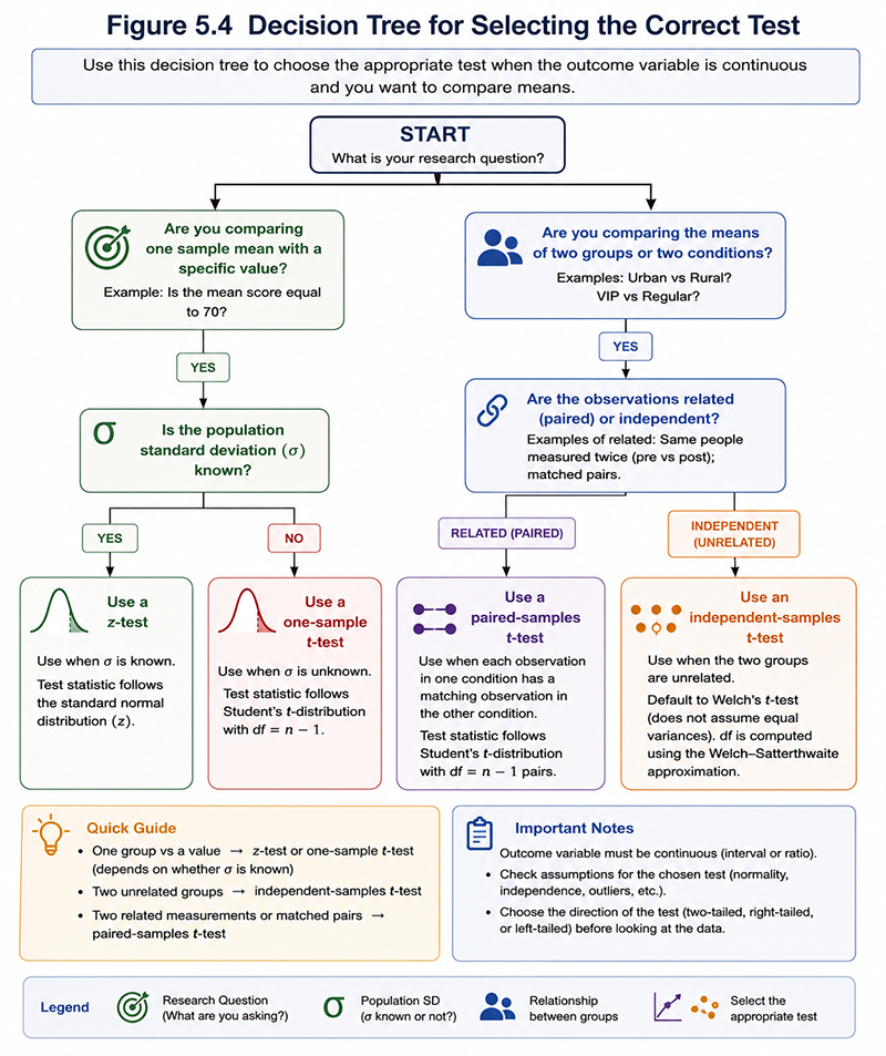
Begin by asking whether the analysis compares means.
After selecting the test, determine whether the hypothesis is two-tailed, right-tailed, or left-tailed. Then check the relevant assumptions, calculate the test statistic, interpret the p-value and confidence interval, examine the effect size, and report the result in context.
A researcher compares the mean Credit Score of 100 customers with a benchmark of 650. The population standard deviation is unknown. Which test should be used?
A one-sample t-test should be used because one sample mean is being compared with a hypothesised value and the population standard deviation is unknown.
A researcher compares mean Purchase Amount between VIP and Regular customers. Each customer belongs to only one group. Which test is appropriate?
An independent-samples t-test is appropriate because a continuous outcome is being compared between two unrelated groups. Welch's t-test may be used as the default procedure.
Customer Satisfaction is measured before and after a website redesign for the same customers. Which test should be used, and which distribution should be checked for normality?
A paired-samples t-test should be used. The normality assumption applies to the distribution of the difference scores:
\[ d_i=X_{\text{Post},i}-X_{\text{Pre},i} \]The pre and post variables do not need to be normally distributed separately.
This module introduced hypothesis testing as a structured method for evaluating statistical evidence. You learned how null and alternative hypotheses are formulated, how significance levels, p-values, critical values, rejection regions, Type I and Type II errors, statistical power, and sample size influence statistical decisions.
The one-sample z-test was introduced as the basic test for comparing a sample mean with a hypothesised population mean when the population standard deviation is known. Because this condition is rarely satisfied in practice, Student's t-distribution was then introduced as the foundation of the one-sample, independent-samples, and paired-samples t-tests.
Across all tests, the same analytical workflow was followed: identify the research question, select the appropriate test, state the hypotheses, assess assumptions, calculate the test statistic, interpret the p-value and confidence interval, evaluate the effect size, and communicate the result using plain language and APA reporting conventions.
The LearnerBox Statistical Explorer reinforced this workflow by showing how changes in hypothesis direction, significance level, group structure, and paired measurements affect the statistical conclusion.
Take a short Quiz and find your score. You can always come back to this page and go through the content again!