

If you find the content useful and wish to support our platform’s development, you can contribute any amount toward our production costs. Scan the UPI QR code for payment within India. Or use the Ko-fi link to process a secure payment via PayPal.
If you find the content useful and wish to support our platform’s development, you can contribute any amount toward our production costs. Scan the UPI QR code for payment within India. Or use the Ko-fi link to process a secure payment via PayPal.
Up to this point in the LearnerBox Statistics series, you have learned how to organise, summarise, and visualise data using both numerical techniques and graphical methods. These skills form the foundation of exploratory data analysis and enable analysts to understand the characteristics of a dataset before drawing conclusions. However, an important question still remains unanswered. How can we use information obtained from a sample to make reliable conclusions about an entire population? Answering this question requires a new branch of statistics known as statistical inference, and statistical inference is built upon the principles of probability.
Probability provides a mathematical framework for describing uncertainty. Every time we collect a sample, measure a variable, or build a predictive model, there is an element of randomness involved. Two random samples drawn from the same population will almost never produce identical results, yet statistical methods allow us to quantify this natural variation and determine how much confidence we can place in our conclusions. Rather than eliminating uncertainty, probability helps us measure and interpret it objectively.
In this module, you will study the probability distributions that form the theoretical foundation of modern statistical analysis. You will learn how random variables behave, why the normal distribution appears so frequently in real-world data, how repeated sampling produces predictable patterns, and why the Central Limit Theorem is regarded as one of the most important results in statistics. These concepts provide the theoretical bridge between descriptive statistics and inferential statistics and prepare you for the hypothesis tests, confidence intervals, regression models, and machine learning techniques that follow in later modules.
Unlike traditional probability courses, this module focuses only on those concepts that are directly relevant to statistical analysis. Our objective is not to derive complex probability formulas but to develop an intuitive understanding of how probability explains the behaviour of data. Throughout the module, emphasis is placed on interpretation, visualisation, and practical application rather than mathematical proof. By the end of this chapter, you will appreciate that probability is not an isolated topic but the language through which statisticians describe uncertainty and make evidence-based decisions.
After completing this module, you should be able to:
One of the defining characteristics of statistics is that it deals with uncertainty. If every member of a population could be observed and measured perfectly, there would be little need for statistical inference. In practice, however, analysts rarely have access to complete populations. Instead, they collect samples and use the information contained within those samples to estimate unknown population characteristics. Because different samples naturally produce different results, uncertainty becomes an unavoidable part of statistical reasoning.
Probability provides the mathematical language for describing this uncertainty. Rather than treating differences between samples as errors or imperfections, probability recognises that variation is a natural consequence of random sampling. It allows statisticians to quantify the likelihood of different outcomes, evaluate competing explanations, and determine whether an observed result is likely to represent a genuine population characteristic or simply random variation. Consequently, probability transforms uncertainty from something that is merely acknowledged into something that can be measured objectively.
The importance of probability extends far beyond traditional statistical analysis. Modern data science, artificial intelligence, finance, healthcare, engineering, and scientific research all rely upon probability models to support evidence-based decision making. Whether predicting customer purchasing behaviour, estimating the effectiveness of a new medical treatment, identifying fraudulent financial transactions, or forecasting future demand, analysts use probability to measure confidence in their conclusions and to communicate the uncertainty associated with every prediction. Understanding probability therefore represents an essential step towards understanding how modern statistical methods—and ultimately many artificial intelligence systems—learn from data.
Almost certainly not.
The difference between these sample averages does not necessarily indicate an error. Instead, it reflects the natural variability that occurs whenever random samples are drawn from a population. The objective of probability theory is to describe and measure this variability so that meaningful statistical conclusions can be drawn despite the presence of uncertainty.
Probability theory is concerned with describing uncertain events in a systematic and measurable way. In statistics, uncertainty is usually associated with the values that variables may assume when observations are collected from a population. Some customers spend more than others, some students obtain higher examination scores, and some manufactured products are defective while others meet quality standards. Although the exact outcome for an individual observation may be uncertain, the overall pattern of possible outcomes often follows a predictable distribution. Understanding these patterns begins with the concept of the random variable.
A random variable is a numerical quantity whose value depends upon the outcome of a random process. Unlike ordinary mathematical variables, the exact value of a random variable is not known in advance. Instead, it takes one of several possible values according to an underlying probability distribution. Random variables provide the connection between probability theory and statistics because they allow uncertainty to be represented numerically and analysed using statistical methods.
Random variables are commonly classified into two broad categories: discrete and continuous. A discrete random variable can assume only specific, countable values. Examples include the number of defective products in a batch, the number of customers making a purchase during a given hour, or the number of students who pass an examination. Because the possible outcomes are countable, discrete random variables are generally analysed using probability distributions such as the binomial distribution.
In contrast, a continuous random variable can assume any value within a specified interval. Examples include customer waiting time, annual income, body temperature, examination scores expressed as percentages, and purchase amounts. Since continuous variables may take infinitely many values, they are described using continuous probability distributions, the most important of which is the normal distribution introduced later in this module.
A useful way to distinguish between these two types of variables is to ask a simple question:
Can the values be counted individually, or are they measured along a continuous scale?
If the values are counted, the variable is usually discrete. If they are measured, the variable is usually continuous. Although this guideline has occasional exceptions, it provides an effective starting point for classifying variables encountered in practical statistical analysis.
A probability distribution describes the possible values that a random variable may assume together with the probability associated with each value. Rather than examining individual observations in isolation, a probability distribution provides a complete picture of how the values of a variable are expected to behave over many repeated observations. Consequently, probability distributions form the mathematical models upon which statistical inference is built.
Different random variables require different probability distributions. For example, the number of customers who purchase a product during an hour may follow a binomial distribution under appropriate conditions, whereas customer satisfaction scores may be approximated by a normal distribution if sufficient observations are collected. Choosing an appropriate probability distribution is therefore an important step in statistical modelling because it determines which analytical techniques may subsequently be applied.
Probability distributions are characterised by several important properties. Every probability distribution assigns a probability to each possible outcome, and the probabilities across all possible outcomes always sum to one. Furthermore, the shape of the distribution provides valuable information about the behaviour of the variable, including where observations are concentrated, how widely they are dispersed, and whether unusually large or unusually small values are likely to occur. Throughout the remainder of this module, you will encounter several probability distributions that illustrate these principles in different ways.
Determine whether each of the following variables should be classified as discrete or continuous.
| Variable | Classification |
|---|---|
| Number of defective products in a shipment | ? |
| Annual income of a customer | ? |
| Number of website visits during one day | ? |
| Customer satisfaction score (0–10) | ? |
| Time required to complete an online purchase | ? |
| Variable | Classification | Reason |
|---|---|---|
| Number of defective products | Discrete | Counted observations |
| Annual income | Continuous | Measured monetary value |
| Website visits | Discrete | Counted events |
| Customer satisfaction score | Continuous (treated as numerical) | Measured rating scale |
| Purchase completion time | Continuous | Measured time interval |
Correctly identifying the type of random variable is an important first step in statistical analysis because it influences the choice of probability distribution, graphical representation, and subsequent statistical techniques.
Among all discrete probability distributions, the binomial distribution is one of the most widely used in statistics. It models situations in which an experiment consists of a fixed number of independent trials, and each trial has only two possible outcomes. These outcomes are commonly referred to as success and failure, although the terms simply distinguish the outcome of interest from every other possible outcome. For example, a customer either makes a purchase or does not, a manufactured component is either defective or non-defective, or a patient either responds to a treatment or does not respond.
The binomial distribution is appropriate only when four conditions are satisfied.
When the assumptions of the binomial distribution are satisfied, the probability of observing exactly x successes in n independent trials is given by the binomial probability function.
| Symbol | Meaning |
|---|---|
| \(P(X=x)\) | Probability of observing exactly \(x\) successes |
| \(n\) | Total number of independent trials |
| \(x\) | Number of successes of interest |
| \(p\) | Probability of success on each trial |
| \(1-p\) | Probability of failure on each trial |
| \(\binom{n}{x}\) | Number of different ways of arranging \(x\) successes among \(n\) trials |
The term
\[ p^x(1-p)^{\,n-x} \]calculates the probability of one particular sequence containing exactly \(x\) successes and \(n-x\) failures. However, those successes and failures may occur in many different orders. The binomial coefficient
\[ \binom{n}{x} = \frac{n!}{x!(n-x)!} \]counts the number of distinct arrangements of these outcomes. Multiplying these two components therefore gives the probability of obtaining exactly \(x\) successes regardless of the order in which they occur.
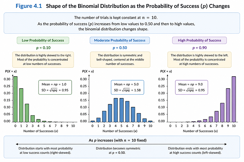
Figure 4.1 demonstrates how the probability of success influences the shape of the binomial distribution. When the probability of success is small, most observations occur near zero successes. As the probability approaches 0.50, the distribution becomes increasingly symmetric. When the probability exceeds 0.50, the distribution shifts towards larger numbers of successes. This illustrates an important principle in probability: changing the underlying probability changes the entire distribution of possible outcomes.
The binomial distribution has numerous practical applications. Businesses use it to estimate the probability that a certain number of customers will respond to a marketing campaign. Manufacturers estimate the number of defective products expected within production batches. Healthcare researchers study the proportion of patients responding to a treatment. Financial analysts estimate the probability of loan defaults, while data scientists frequently model binary outcomes when developing classification algorithms.
Although modern statistical software can calculate binomial probabilities instantly, understanding the assumptions underlying the distribution is far more important than memorising formulas. Before selecting a probability model, analysts should always ask whether the observed data genuinely satisfy the assumptions required by that model.
Suppose a marketing campaign has a response rate of 20%. If emails are sent to 10 randomly selected customers, how does changing the probability of response affect the distribution of the expected number of responses?
Open the LearnerBox Statistical Explorer and select the Distribution Explorer.
Choose:
Observe the resulting probability distribution. Then repeat the analysis using:
Compare the resulting graphs.
As the probability of success increases, the distribution shifts progressively towards larger numbers of successes. When the probability equals 0.50, the distribution becomes approximately symmetric because success and failure are equally likely. This interactive exploration demonstrates that probability distributions are dynamic models whose shapes depend directly upon their underlying parameters.
Among all probability distributions used in statistics, none is more important than the normal distribution. It appears throughout the natural sciences, engineering, economics, medicine, psychology, finance, and artificial intelligence. Many naturally occurring measurements—including human height, blood pressure, examination scores, manufacturing tolerances, and measurement errors—are often found to approximate a normal distribution when sufficiently large samples are collected. Even when the original data are not normally distributed, the Central Limit Theorem, introduced later in this module, explains why the normal distribution continues to play a central role in statistical inference.
The normal distribution is frequently referred to as the Gaussian distribution or the bell-shaped distribution because of its distinctive symmetric shape. Unlike the discrete binomial distribution, which describes probabilities associated with countable outcomes, the normal distribution models continuous variables that may assume infinitely many values within a specified range. Rather than assigning probabilities to individual observations, it describes how probability is distributed continuously across all possible values of the variable.
One of the most remarkable characteristics of the normal distribution is that its shape is determined entirely by two parameters: the population mean (\(\mu\)) and the population standard deviation (\(\sigma\)). The mean determines the location of the centre of the distribution, while the standard deviation determines the amount of dispersion around the mean. Changing either parameter alters the appearance of the distribution without changing its fundamental bell-shaped form.
Because of its importance, the normal distribution is used extensively throughout statistics. Confidence intervals, hypothesis tests, regression analysis, quality control procedures, forecasting models, and numerous machine learning algorithms either assume normality directly or rely upon results derived from the normal distribution. Understanding its properties therefore provides the conceptual foundation for much of the remainder of this textbook.
The mathematical model describing the normal distribution is known as the normal probability density function.
\[ f(x)= \frac{1}{\sigma\sqrt{2\pi}} \exp\left[ -\frac{(x-\mu)^2}{2\sigma^2} \right] \]| Symbol | Meaning |
|---|---|
| \(x\) | Observed value of the variable |
| \(\mu\) | Population mean |
| \(\sigma\) | Population standard deviation |
| \(\pi\) | Mathematical constant (approximately 3.14159) |
| \(e\) | Base of the natural logarithm (approximately 2.71828) |
| \(f(x)\) | Probability density at the value \(x\) |
Unlike the binomial probability function, the normal probability density function does not calculate the probability of observing one exact value. Because continuous variables may assume infinitely many values, the probability of observing any single value is effectively zero. Instead, probabilities are obtained by calculating the area under the curve between two values. Consequently, the normal distribution is interpreted geometrically: larger areas correspond to higher probabilities, while smaller areas correspond to lower probabilities.
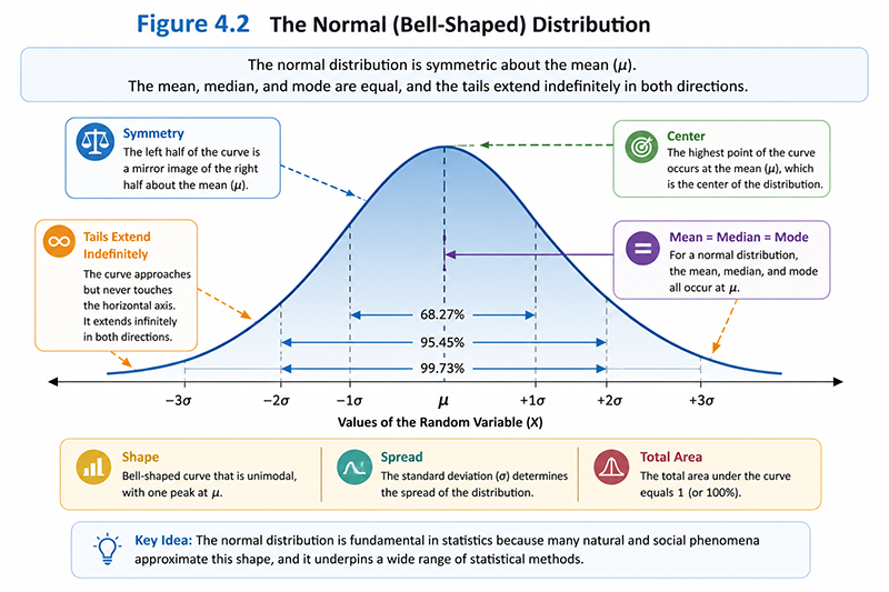
Figure 4.2 illustrates the characteristic bell-shaped curve of the normal distribution. Several important properties can be observed immediately. First, the distribution is perfectly symmetric about the mean, implying that observations are equally likely to occur above or below the centre. Second, the mean, median, and mode coincide at the same location, reflecting the absence of skewness. Third, although the curve becomes increasingly close to the horizontal axis towards both extremes, it never actually touches the axis. These tails represent the possibility of observing increasingly extreme values, although such observations become progressively less probable.
The total area beneath the normal curve is equal to one, representing the complete probability associated with all possible outcomes. Consequently, every probability calculated from the normal distribution corresponds to the area enclosed beneath the curve between specified values. This simple geometric interpretation allows statisticians to visualise probabilities rather than treating them as abstract numerical quantities.
One of the most useful properties of the normal distribution is that the proportion of observations within specific distances from the mean remains remarkably consistent. This relationship is known as the Empirical Rule, the 68–95–99.7 Rule, or the Three-Sigma Rule. It provides a convenient method for estimating the proportion of observations that lie within one, two, and three standard deviations of the mean without performing detailed probability calculations.
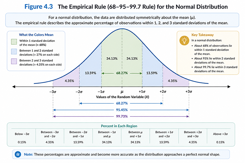
Figure 4.3 illustrates the Empirical Rule for the normal distribution. Approximately 68% of all observations lie within one standard deviation of the mean \((\mu \pm \sigma)\), approximately 95% lie within two standard deviations \((\mu \pm 2\sigma)\), and approximately 99.7% lie within three standard deviations \((\mu \pm 3\sigma)\). Consequently, observations occurring more than three standard deviations from the mean are relatively uncommon and often warrant further investigation.
The Empirical Rule provides valuable insight into the variability of normally distributed data. For example, suppose the examination scores of a large group of students are approximately normally distributed with a mean of 70 and a standard deviation of 10. The rule suggests that approximately 68% of students would obtain scores between 60 and 80, approximately 95% would score between 50 and 90, and almost all students would obtain scores between 40 and 100. Without performing any formal probability calculations, the analyst is therefore able to estimate the likely distribution of observations within the population.
The Empirical Rule also provides an intuitive method for identifying unusual observations. Values lying beyond three standard deviations from the mean occur very infrequently in a normal distribution. Such observations are not necessarily incorrect, but they deserve careful examination because they may represent measurement errors, data entry mistakes, or genuinely exceptional cases. In later modules, this principle will assist in identifying potential outliers and evaluating the assumptions underlying statistical models.
Suppose customer satisfaction scores are approximately normally distributed with a mean of 80 and a standard deviation of 5.
Use the Empirical Rule to estimate the proportion of customers whose satisfaction scores fall:
Open the LearnerBox Statistical Explorer and select the Distribution Explorer.
Set:
Use the Empirical Rule tab to highlight the regions corresponding to one, two, and three standard deviations.
The estimated proportions are:
The Empirical Rule allows analysts to estimate probabilities directly from the normal distribution without consulting probability tables or performing detailed calculations. Although the percentages are approximate, they are remarkably accurate for variables that closely follow a normal distribution.
Although every normal distribution has the same bell-shaped form, different variables may have very different means and standard deviations. For example, annual income may have a mean of ₹650,000 and a standard deviation of ₹150,000, whereas examination scores may have a mean of 72 and a standard deviation of 8. Because these variables are measured on completely different scales, comparing individual observations directly is often difficult.
Statisticians solve this problem by converting observations from their original measurement scale to a common standard scale. This process is known as standardisation. Once a variable has been standardised, its values indicate how far each observation lies above or below the mean in units of standard deviation rather than in the original measurement units.
The resulting distribution is called the standard normal distribution. Unlike an ordinary normal distribution, the standard normal distribution always has:
Because every normally distributed variable can be transformed into this common scale, statisticians are able to compare observations originating from entirely different populations and measurement systems. Standardisation therefore plays an important role throughout statistical inference and machine learning.
The standardised value of an observation is known as its z-score. A z-score measures the number of standard deviations by which an observation differs from the population mean.
| Symbol | Meaning |
|---|---|
| \(z\) | Standardised score |
| \(x\) | Observed value |
| \(\mu\) | Population mean |
| \(\sigma\) | Population standard deviation |
The numerator \((x-\mu)\) measures how far the observation lies from the population mean. Dividing this difference by the population standard deviation expresses the distance in standard deviation units rather than the original measurement units.
Consequently,
Because all standard normal distributions share the same scale, z-scores allow observations from completely different variables to be compared directly.
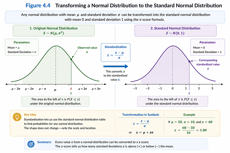
Figure 4.4 illustrates the process of transforming an observation from its original measurement scale to the standard normal scale. Regardless of whether the original variable measures income, examination scores, customer satisfaction, or product weight, standardisation expresses every observation using the same reference system. This common scale allows probabilities, percentiles, and statistical comparisons to be interpreted consistently across different datasets.
A student obtains an examination score of 82 in a course where the class mean is 70 and the population standard deviation is 8.
Calculate the student's z-score and interpret the result.
Substituting the values into the formula:
\[ z=\frac{x-\mu}{\sigma} = \frac{82-70}{8} = \frac{12}{8} = 1.50 \]The student's examination score is therefore
\[ z=1.50 \]The student scored 1.5 standard deviations above the class mean. Referring to the standard normal distribution, this indicates that the student's performance was substantially above average.
Using the LearnerBox Statistical Explorer, enter the values:
Observe how the corresponding point is highlighted on both the original normal distribution and the standard normal distribution.
Throughout this module, we have studied probability distributions that describe the behaviour of individual observations. However, statistical inference is rarely based upon individual observations alone. Instead, analysts usually collect a sample and calculate one or more sample statistics, such as the sample mean, sample proportion, or sample standard deviation. This naturally raises an important question.
How do sample statistics behave when different random samples are drawn from the same population?
The answer lies in the concept of the sampling distribution.
A sampling distribution is the probability distribution of a statistic calculated from all possible random samples of a fixed size drawn from the same population. Rather than describing the behaviour of individual observations, a sampling distribution describes the behaviour of an estimator. In practice, the most important sampling distribution is the distribution of the sample mean.
To understand this idea, imagine a population containing thousands of customers. Drawing one random sample of 50 customers produces one sample mean. Drawing another random sample of 50 customers usually produces a slightly different mean because different individuals have been selected. If this sampling process were repeated hundreds or thousands of times, the resulting sample means would themselves form a distribution. This new distribution is called the sampling distribution of the mean.
Several important properties distinguish a sampling distribution from the original population distribution.
The spread of the sampling distribution is measured by the standard error of the mean, which is given by
\[ SE_{\bar{x}} = \frac{\sigma}{\sqrt{n}} \]where
| Symbol | Meaning |
|---|---|
| \(SE_{\bar{x}}\) | Standard error of the sample mean |
| \(\sigma\) | Population standard deviation |
| \(n\) | Sample size |
The standard error measures the expected variability of sample means obtained from repeated random sampling. As the sample size increases, the denominator becomes larger, causing the standard error to decrease. Consequently, larger samples tend to produce more stable and more precise estimates of the population mean.
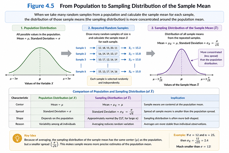
Figure 4.5 illustrates the relationship between a population and the corresponding sampling distribution of the sample mean. Although individual observations may vary substantially, repeated sampling produces sample means that cluster much more closely around the population mean. This reduction in variability explains why averaging observations provides a more stable estimate of the underlying population characteristic than relying upon individual measurements.
Using the LearnerBox Statistical Explorer, investigate how increasing the sample size influences the sampling distribution of the sample mean.
Open the Sampling Explorer and choose:
Run the simulation using:
Observe the resulting sampling distributions.
As the sample size increases, the sampling distribution becomes progressively narrower because the standard error decreases. Although the original population remains unchanged, larger samples produce more precise estimates of the population mean.
Among all results in statistics, the Central Limit Theorem (CLT) is perhaps the most important. It provides the theoretical explanation for why so many statistical methods work and forms the foundation of confidence intervals, hypothesis testing, regression analysis, analysis of variance, and many predictive modelling techniques.
The Central Limit Theorem states that, regardless of the shape of the original population distribution, the sampling distribution of the sample mean approaches a normal distribution as the sample size becomes sufficiently large, provided that random sampling has been used and the observations are independent.
This result is remarkable because the original population does not need to be normally distributed. The population may be positively skewed, negatively skewed, uniform, or even bimodal. As increasingly large random samples are drawn, the distribution of the sample means nevertheless becomes approximately normal.
The Central Limit Theorem explains why the normal distribution appears throughout inferential statistics. Even when real-world data do not follow a perfect bell-shaped distribution, the sampling distributions of many commonly used statistics become approximately normal for sufficiently large samples. Consequently, probability calculations based upon the normal distribution remain valid for a wide range of practical applications.
Use the LearnerBox Statistical Explorer to investigate the Central Limit Theorem.
Within the Sampling Explorer, choose several different population shapes:
For each population, repeatedly generate sampling distributions using:
Observe how the distribution of the sample means changes as the sample size increases.
Although the original populations remain very different, the sampling distributions gradually become bell-shaped as the sample size increases. This simulation demonstrates visually one of the most powerful ideas in statistics: repeated sampling transforms highly variable populations into remarkably predictable sampling distributions.
Throughout this module, we have explored how probability distributions describe uncertainty, how the normal distribution models continuous variables, and how repeated random sampling produces predictable sampling distributions. These ideas are not isolated mathematical concepts. Together, they provide the theoretical foundation upon which statistical inference is built.
Statistical inference seeks to answer an important practical question:
How can information obtained from a sample be used to draw conclusions about an entire population?
Because every sample differs slightly from every other sample, a single sample statistic is never expected to equal the corresponding population parameter exactly. Instead of attempting to identify one exact population value, statisticians estimate a range of plausible values within which the true population parameter is likely to lie. This range is known as a confidence interval.
A confidence interval (CI) combines three important pieces of information:
Together, these quantities produce an interval that is likely to contain the unknown population parameter.
For example, suppose a survey estimates that the average monthly expenditure of customers is $30,000 with a 95% confidence interval ranging from $28,800 to ₹31,200. Rather than claiming that the true population mean is exactly $30,000, the analyst concludes that the available evidence suggests the population mean is likely to lie somewhere within this interval. The confidence interval therefore communicates both the estimated value and the uncertainty associated with that estimate.
The confidence level reflects the long-run performance of the estimation procedure. A 95% confidence interval does not mean that there is a 95% probability that the particular interval calculated from one sample contains the population parameter. Instead, it means that if the same sampling procedure were repeated many times, approximately 95% of the resulting confidence intervals would contain the true population parameter.
This interpretation depends directly upon the Central Limit Theorem introduced in the previous section. Because repeated sample means follow an approximately normal distribution, probability can be used to determine how far sample estimates are expected to vary from the true population parameter. Consequently, confidence intervals provide a practical application of probability theory to statistical estimation.
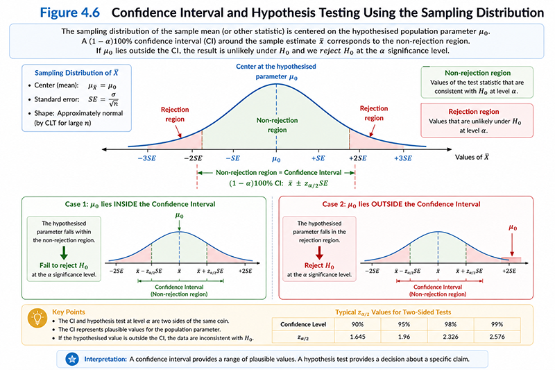
Figure 4.6 illustrates the relationship between confidence intervals and statistical decision making. If the hypothesised population value falls within the confidence interval, the observed sample result is considered consistent with the null hypothesis, and there is insufficient evidence to reject it. Conversely, if the hypothesised value lies outside the confidence interval, the sample result is considered unlikely under the null hypothesis, providing evidence in favour of rejecting it.
Although confidence intervals and hypothesis tests are often presented as separate statistical procedures, they are closely related. In many situations, they lead to exactly the same conclusion because both rely upon the same sampling distribution, the same standard error, and the same underlying probability model. Confidence intervals emphasise estimation, whereas hypothesis tests emphasise decision making.
A company estimates that the average monthly purchase amount of its customers is ₹30,500. A 95% confidence interval is calculated as:
\[ 29,700 \le \mu \le 31,300 \]The marketing department believes that the true average monthly purchase amount is ₹32,000.
Based solely on the confidence interval, what statistical conclusion can be drawn?
Open the LearnerBox Statistical Explorer and select the Confidence Interval Explorer.
Enter:
Observe the position of the hypothesised value relative to the confidence interval.
Because ₹32,000 lies outside the confidence interval, the hypothesised value is not consistent with the observed sample at the 95% confidence level. Consequently, there is sufficient evidence to reject the null hypothesis that the population mean equals ₹32,000.
The annual incomes of employees in a company are approximately normally distributed with a population mean of ₹600,000 and a population standard deviation of ₹80,000.
Calculate the z-score for an employee whose annual income is ₹720,000.
Using the z-score formula,
\[ z=\frac{x-\mu}{\sigma} \]Substituting the values,
\[ z=\frac{720000-600000}{80000} =\frac{120000}{80000} =1.50 \]Therefore,
\[ z=1.50 \]The employee's income is 1.5 standard deviations above the population mean. This indicates that the employee earns substantially more than the average employee within the organisation.
Two students take different examinations.
| Student | Examination Score | Mean | Standard Deviation |
|---|---|---|---|
| A | 82 | 70 | 8 |
| B | 91 | 80 | 5 |
A random sample of customers produces a sample mean monthly expenditure of ₹12,500.
The standard error of the mean is ₹400.
Construct a 95% confidence interval for the population mean using the approximation
\[ \bar{x}\pm1.96(SE) \]Margin of error:
\[ 1.96\times400 =784 \]Lower limit:
\[ 12500-784 =11716 \]Upper limit:
\[ 12500+784 =13284 \]Therefore,
\[ 95\% \text{ CI} = (11,716,\;13,284) \]The analyst estimates that the true population mean monthly expenditure is likely to lie between ₹11,716 and ₹13,284.
A manufacturer claims that the average lifetime of a battery is 500 hours.
A 95% confidence interval calculated from a random sample is
\[ (512,\;548) \]Evaluate the manufacturer's claim using the confidence interval.
The hypothesised value
\[ 500 \]lies outside the confidence interval
\[ (512,\;548) \]Using the LearnerBox Statistical Explorer, enter:
Observe the location of the hypothesised value relative to the interval.
Because the claimed population mean lies outside the confidence interval, the sample evidence is inconsistent with the manufacturer's claim at the 95% confidence level.
Consequently, there is sufficient statistical evidence to reject the claim that the average battery lifetime equals 500 hours.
1. Explain the difference between a discrete random variable and a continuous random variable.
2. Why is the normal distribution considered one of the most important probability distributions in statistics?
3. Explain the Empirical Rule (68–95–99.7 Rule) in your own words.
4. Distinguish between a population distribution and a sampling distribution.
5. Why is the Central Limit Theorem regarded as the foundation of statistical inference?
1. Calculate the z-score for an examination score of 88 when the class mean is 75 and the standard deviation is 6.
2. A product weighs 2.35 kg. The population mean is 2.20 kg and the population standard deviation is 0.10 kg. Calculate and interpret the corresponding z-score.
3. Construct a 95% confidence interval for a sample mean of 46.2 when the standard error is 1.4.
4. A confidence interval for the population mean is (98.4, 103.6). Can the hypothesis that the population mean equals 100 be rejected at the 95% confidence level? Explain your reasoning.
1. Using the Distribution Explorer, investigate how changing the probability of success (p) alters the shape of the binomial distribution.
2. Using the Distribution Explorer, vary the mean and standard deviation of the normal distribution. Describe how each parameter changes the position and spread of the curve.
3. Using the Sampling Explorer, compare the sampling distributions obtained for sample sizes of 5, 30, and 100. Explain how increasing the sample size affects the standard error.
4. Using the Confidence Interval Explorer, investigate how changing the confidence level influences the width of the confidence interval.
5. Place several hypothesised population values inside and outside a confidence interval. Describe how the statistical decision changes.
In this module, you explored the probabilistic foundations of statistical inference. Beginning with random variables and probability distributions, you learned how uncertainty can be represented mathematically and how different probability models describe different types of data. You then examined the binomial distribution for discrete outcomes and the normal distribution for continuous variables, together with the Empirical Rule and the concept of standardisation through z-scores.
Building upon these ideas, you investigated sampling distributions and discovered how repeated random sampling produces predictable statistical behaviour. The Central Limit Theorem demonstrated why the sampling distribution of the sample mean approaches normality, regardless of the shape of the original population. Finally, you learned how these principles lead naturally to confidence intervals, providing the theoretical bridge from descriptive statistics to statistical inference.
The concepts introduced in this module form the mathematical foundation for the remainder of the LearnerBox Statistics series. In the next module, you will apply these ideas to hypothesis testing, where probability is used to evaluate research questions and make evidence-based decisions about populations using sample data.
Take a short Quiz and find your score. You can always come back to this page and go through the content again!