

AI Skills Cookbook
Intermediate
10 min read
From ML to DL with PyTorch
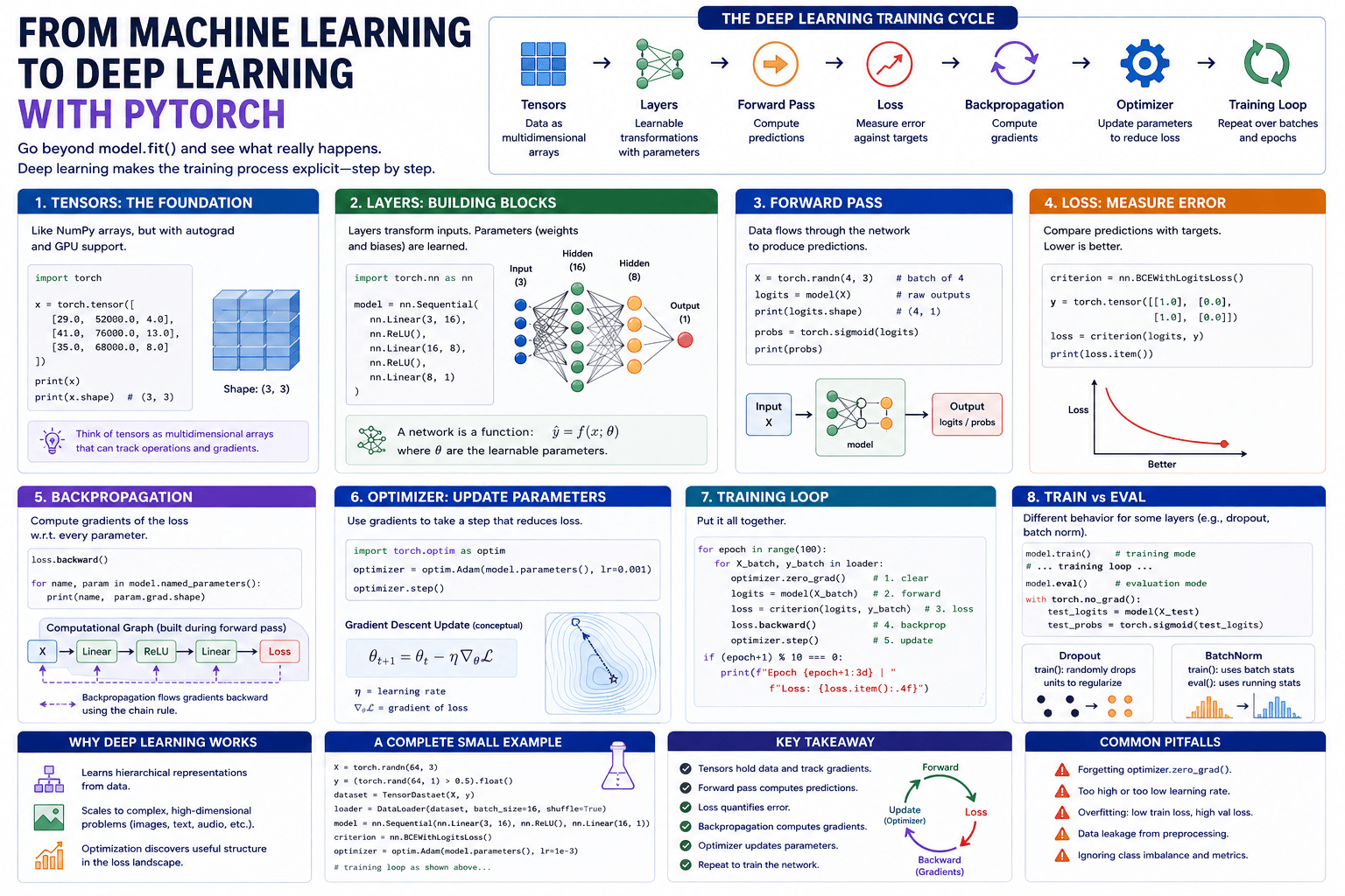
Discover how PyTorch reveals the mechanics of deep learning, from tensors and neural network layers to forward passes, loss, backpropagation, and the training loops that enable models to learn.
Introduction
In the previous AI Skills Cookbook guide, we built a complete machine learning workflow with scikit-learn. After preparing the data and defining a pipeline, training the model eventually came down to a deceptively simple instruction:
model.fit(X_train, y_train)That abstraction is enormously useful. But it conceals almost everything involved in learning. Somewhere underneath .fit(), predictions must be calculated, those predictions must be compared with the correct answers, the resulting error must be translated into information about how the model should change, and its parameters must then be updated. This process must happen repeatedly until the model learns a useful mapping from inputs to outputs.
Deep learning makes this machinery much more visible. Frameworks such as PyTorch still automate the difficult numerical operations, but they expose the fundamental components of learning: tensors, layers, parameters, forward passes, loss functions, gradients, backpropagation, optimizers, and training loops.
The conceptual progression is:
Tensors → Layers → Forward Pass → Loss → Backpropagation → Optimizer → Training Loop
Understanding this cycle is far more important than memorizing PyTorch syntax. Once the cycle becomes intuitive, neural networks stop appearing as mysterious systems that somehow "learn" and instead become understandable computational models whose parameters are repeatedly adjusted to reduce prediction error.
From Arrays to Tensors
The transition from NumPy to PyTorch begins with a familiar idea. In NumPy, numerical information is represented using multidimensional arrays. PyTorch uses tensors, which provide a closely related abstraction but add capabilities required for neural networks, particularly automatic differentiation and accelerator-based computation.
A tensor can be created directly:
import torch

x = torch.tensor([
    [29.0, 52000.0, 4.0],
    [41.0, 76000.0, 13.0],
    [35.0, 68000.0, 8.0]
])

print(x)
print(x.shape)
print(x.dtype)
The shape here is (3, 3): three observations and three features. As in the previous guide, we can think of this as a feature matrix
where $n$ is the number of observations and $p$ is the number of input features.
But tensors extend naturally into higher dimensions. A batch of color images may have dimensions corresponding to batch size, channels, height, and width. Language models manipulate tensors representing batches of token sequences and high-dimensional embeddings. The same conceptual structure therefore scales from a simple tabular dataset to enormous transformer networks.
Tensors can also be moved between computational devices:
device = torch.device(
    "cuda" if torch.cuda.is_available() else "cpu"
)

x = x.to(device)

print(device)
This is one reason tensor frameworks became central to deep learning: the mathematical operations used by neural networks can be executed efficiently on GPUs and other accelerators without rewriting the model in a low-level programming language.
Neural Networks as Functions
A neural network can be understood as a parameterized mathematical function.
For a simple linear layer,
\[z = XW + b\]where $X$ contains the inputs, $W$ contains learned weights, and $b$ contains learned biases. The values in $W$ and $b$ are the model's parameters.
A neural network becomes more expressive when several transformations are composed together. A simple two-layer network might be represented as
\[h = \text{ReLU}(XW_1 + b_1)\]followed by
\[\hat{y} = hW_2 + b_2\]The first transformation produces a hidden representation $h$. The nonlinear ReLU activation allows the network to model relationships that cannot be expressed by a single linear transformation. The second layer converts that hidden representation into an output.
In PyTorch, the same architecture can be written using torch.nn:
import torch.nn as nn

model = nn.Sequential(
    nn.Linear(3, 16),
    nn.ReLU(),
    nn.Linear(16, 1)
)

print(model)
The input contains three features. The first layer maps those three values into a 16-dimensional hidden representation, ReLU introduces nonlinearity, and the final layer produces one output.
This small network contains the same fundamental ingredients found in much larger deep learning systems. Modern architectures may contain billions of parameters and enormously more sophisticated layers, but they remain compositions of differentiable transformations whose parameters are learned from data.
What Makes a Network "Deep"?
A network becomes deep when multiple learned layers are composed so that information passes through a hierarchy of transformations.
Instead of learning a single mapping from input to output, the network progressively constructs intermediate representations:
\[X \to h_1 \to h_2 \to h_3 \to \cdots \to \hat{y}\]These representations are one reason deep learning became so powerful. In computer vision, earlier layers may respond to relatively simple visual structures while deeper layers can represent increasingly complex patterns. In language models, token representations are repeatedly transformed through attention and feed-forward layers, allowing contextual relationships to emerge across many levels of computation.
This connects directly with Interpretability & Representation Engineering from The Science of AI. Neural networks do not merely store answers. During training, they develop distributed internal representations that help them perform the task for which they are being optimized.
The architecture determines which kinds of transformations are easy or difficult for the model to learn, connecting equally strongly with Inductive Biases & Architecture Limits. Deep learning therefore does not eliminate assumptions about model design; it embeds those assumptions within architecture.
The Forward Pass: Turning Inputs into Predictions
Once the network has been defined, data can be passed through it:
X = torch.tensor([
    [0.2, -0.4, 0.7],
    [0.8, 0.1, -0.2],
    [-0.3, 0.6, 0.4]
], dtype=torch.float32)

logits = model(X)

print(logits)
This computation is called the forward pass.
Each layer receives the output of the preceding layer, applies its mathematical transformation, and passes the result onward. Eventually, the final layer produces the model's prediction or, depending on the architecture and loss function, a quantity from which a prediction can be derived.
For binary classification, the raw final output is often called a logit. A sigmoid function can transform a logit $z$ into a probability:
\[\sigma(z) = \frac{1}{1+e^{-z}}\]In PyTorch:
probabilities = torch.sigmoid(logits)If the resulting probability is 0.91, the model is assigning a much stronger belief to the positive class than if the probability were 0.53.
However, during training we usually do not manually apply the sigmoid when using BCEWithLogitsLoss, because that loss combines the sigmoid transformation and binary cross-entropy in a numerically stable implementation.
That small implementation detail illustrates an important characteristic of advanced framework use: understanding the mathematics helps us choose the correct abstraction rather than reproducing every mathematical step manually.
Loss: Converting Error into an Objective
Producing a prediction is not enough. The model needs a way to determine how wrong that prediction is.
A loss function converts the difference between predictions and targets into a scalar quantity that training attempts to minimize.
For binary classification, binary cross-entropy can be written as
\[\mathcal{L} = -\frac{1}{N}\sum_{i=1}^N \left[y_i \log(p_i) + (1-y_i)\log(1-p_i)\right]\]where $y_i$ is the true class and $p_i$ is the predicted probability.
In PyTorch:
criterion = nn.BCEWithLogitsLoss()

y = torch.tensor([
    [1.0],
    [0.0],
    [1.0]
])

loss = criterion(logits, y)

print(loss.item())
The loss is not simply a report card generated after training. It is the mathematical objective that drives learning itself. The optimizer needs to know how changing each parameter would affect this quantity.
This brings us to the mechanism that makes modern neural network training possible.
Gradients: Which Direction Should the Model Move?
Suppose the model contains parameters
\[\theta = \{W_1, b_1, W_2, b_2, \ldots\}\]and the loss is a function of those parameters:
\[\mathcal{L}(\theta)\]To reduce the loss, we want to know how sensitive it is to each parameter. This information is contained in the gradient:
\[\nabla_\theta \mathcal{L}\]For an individual parameter $\theta_j$, the partial derivative
\[\frac{\partial \mathcal{L}}{\partial \theta_j}\]describes how a small change in that parameter affects the loss.
If the gradient is positive, moving the parameter in one direction increases the loss; moving in the opposite direction tends to decrease it. If the gradient is negative, the direction reverses.
This connects directly with Generalization & the Loss Landscape. Training can be visualized conceptually as moving through a high-dimensional landscape in which each location corresponds to a particular parameter configuration and the height represents loss.
The challenge is that a modern neural network may contain millions or billions of parameters. Calculating every derivative manually would be impractical.
PyTorch solves this through automatic differentiation.
Autograd and Backpropagation
PyTorch records operations performed on tensors that require gradients, constructing a dynamic computational graph. When the final loss is calculated, the framework can traverse this graph backward and apply the chain rule to determine how each parameter contributed to the result.
The entire backward computation is initiated with:
loss.backward()That single line performs backpropagation.
Backpropagation is sometimes described vaguely as "sending the error backward through the network." A more precise description is that it efficiently applies the chain rule through the sequence of differentiable operations used during the forward pass.
If
\[x \to h_1 \to h_2 \to \mathcal{L}\]then the derivative of the loss with respect to an earlier quantity involves products of local derivatives:
\[\frac{\partial \mathcal{L}}{\partial x} = \frac{\partial \mathcal{L}}{\partial h_2}\frac{\partial h_2}{\partial h_1}\frac{\partial h_1}{\partial x}\]The computational graph allows PyTorch to perform this process efficiently across complex architectures.
After calling backward(), the parameters contain gradients:
for name, parameter in model.named_parameters():
    print(name, parameter.grad)
At this stage, the model knows which direction its parameters should move—but they have not yet changed.
The Optimizer: Turning Gradients into Learning
An optimizer uses gradients to update model parameters.
The simplest conceptual update is gradient descent:
\[\theta_{t+1} = \theta_t - \eta \nabla_\theta \mathcal{L}\]where $\eta$ is the learning rate.
The learning rate controls the size of each update. If it is too small, training may progress extremely slowly. If it is too large, parameter updates may overshoot useful regions of the loss landscape or make training unstable.
PyTorch provides several optimizers. Adam is widely used:
import torch.optim as optim

optimizer = optim.Adam(
    model.parameters(),
    lr=0.001
)
An optimizer does not determine what the model should learn; the loss function provides that objective. The optimizer determines how the model navigates parameter space in pursuit of that objective.
This distinction is important. Architecture, loss function, optimizer, learning rate, training data, and initialization all influence learning in different ways.
The Training Loop: Where Deep Learning Actually Happens
We can now assemble the entire mechanism.
for epoch in range(100):

    # 1. Clear old gradients
    optimizer.zero_grad()

    # 2. Forward pass
    logits = model(X)

    # 3. Compute loss
    loss = criterion(logits, y)

    # 4. Backpropagation
    loss.backward()

    # 5. Update parameters
    optimizer.step()

    if (epoch + 1) % 10 == 0:
        print(
            f"Epoch {epoch + 1:3d} | "
            f"Loss: {loss.item():.4f}"
        )
These five operations are the heart of neural network training.
The model begins with parameters that are typically initialized without knowledge of the specific task. The forward pass produces predictions. The loss measures their quality. Backpropagation calculates gradients. The optimizer updates parameters. The next forward pass therefore uses a slightly different model.
Repeated thousands or millions of times across batches of training data, this simple cycle produces the complex representations associated with deep learning.
Forward → Loss → Backward → Update → Repeat
That is what was hidden behind .fit().
zero_grad() → forward → loss → backward() → step(), more advanced abstractions become much easier to reason about and debug.
Why Gradients Must Be Reset
One line in the training loop deserves particular attention:
optimizer.zero_grad()PyTorch accumulates gradients by default. Calling loss.backward() adds newly calculated gradients to those already stored in each parameter rather than automatically replacing them.
This behavior is useful for techniques such as gradient accumulation, but it means that ordinary training loops must clear previous gradients before calculating the next update.
Forgetting this step can cause the optimizer to use accumulated information from several backward passes unintentionally.
This illustrates why understanding the mechanics matters. A training loop can execute without producing an obvious Python error while still implementing the wrong learning procedure.
Mini-Batches and DataLoaders
Real datasets are usually too large—and often computationally undesirable—to process as one enormous tensor during every update. Neural networks are therefore commonly trained using mini-batches.
Suppose the dataset contains $N$ observations. Instead of computing the loss over all $N$ examples before every update, we divide the data into smaller batches:
\[B_1, B_2, \ldots, B_k\]Each batch produces an estimate of the gradient, and the optimizer updates the model repeatedly as it moves through the dataset.
PyTorch provides Dataset and DataLoader abstractions for this purpose:
from torch.utils.data import TensorDataset, DataLoader

dataset = TensorDataset(X, y)

loader = DataLoader(
    dataset,
    batch_size=32,
    shuffle=True
)
The training loop then operates over batches:
for epoch in range(100):

    for X_batch, y_batch in loader:

        optimizer.zero_grad()

        logits = model(X_batch)
        loss = criterion(logits, y_batch)

        loss.backward()
        optimizer.step()
An epoch represents one complete traversal of the training dataset, while an iteration or training step generally represents one parameter update.
Mini-batch training is computationally efficient and introduces stochasticity into optimization. This stochastic behavior is not merely an inconvenience; it can influence which regions of the loss landscape the model explores and may affect generalization.
Training Mode and Evaluation Mode
Deep learning introduces another distinction that does not always appear explicitly in simpler machine learning workflows.
During training:
model.train()During evaluation:
model.eval()For the simple network used above, the distinction may not change anything. But layers such as dropout and batch normalization behave differently during training and inference.
Evaluation should also avoid constructing unnecessary gradient information:
model.eval()

with torch.no_grad():
    test_logits = model(X_test_tensor)
    test_probabilities = torch.sigmoid(test_logits)
This reduces memory usage and computational overhead.
The larger principle remains identical to the previous guide: training and evaluation are different phases with different informational boundaries.
Deep learning does not remove the need for train/validation/test separation, careful preprocessing, appropriate metrics, or leakage prevention. It makes those practices even more important because highly flexible neural networks can exploit subtle patterns extremely effectively.
A Complete Small Neural Network
Putting the major components together gives us a compact but genuine deep learning workflow:
import torch
import torch.nn as nn
from torch.utils.data import TensorDataset, DataLoader

# Reproducibility
torch.manual_seed(42)

# Model
model = nn.Sequential(
    nn.Linear(3, 16),
    nn.ReLU(),
    nn.Linear(16, 8),
    nn.ReLU(),
    nn.Linear(8, 1)
)

# Objective and optimizer
criterion = nn.BCEWithLogitsLoss()

optimizer = torch.optim.Adam(
    model.parameters(),
    lr=0.001
)

# Data loader
dataset = TensorDataset(X_train_tensor, y_train_tensor)

loader = DataLoader(
    dataset,
    batch_size=32,
    shuffle=True
)

# Training
for epoch in range(100):

    model.train()
    running_loss = 0.0

    for X_batch, y_batch in loader:

        optimizer.zero_grad()

        logits = model(X_batch)
        loss = criterion(logits, y_batch)

        loss.backward()
        optimizer.step()

        running_loss += loss.item()

    if (epoch + 1) % 10 == 0:
        mean_loss = running_loss / len(loader)
        print(
            f"Epoch {epoch + 1:3d} | "
            f"Loss: {mean_loss:.4f}"
        )
Despite its modest size, this code contains the essential architecture of deep learning training. Larger systems add complexity through more sophisticated architectures, distributed computation, learning-rate schedules, regularization, mixed-precision training, checkpointing, and extensive evaluation—but the fundamental cycle remains recognizable.
What the Loss Curve Can (and Cannot) Tell You
During training, we often record loss across epochs. A decreasing training loss tells us that optimization is succeeding at its immediate objective: the network is becoming better at fitting the training data.
It does not prove that the model is becoming better at generalization.
A model may continue reducing training loss while validation performance begins deteriorating. That is one manifestation of overfitting. For this reason, serious training workflows monitor both training and validation behavior.
Conceptually, we might observe:
Epoch       Training Loss       Validation Loss
1           0.68                0.69
10          0.51                0.54
20          0.39                0.43
30          0.27                0.41
40          0.18                0.47
At epoch 40, the model has become substantially better at fitting its training examples while becoming worse on unseen validation data.
The lowest training loss is therefore not automatically the best model.
This is another connection to Generalization & the Loss Landscape: optimization and generalization are related, but they are not the same problem.
Why Deep Learning Needs Scale
If neural networks require more complicated training procedures than traditional machine learning models, why use them?
Their advantage becomes particularly important when the data is high-dimensional, abundant, and structurally complex. Images, audio, video, natural language, and large multimodal datasets contain patterns that are difficult to represent through manually engineered features alone.
Deep networks can learn useful representations directly from data.
This capability, however, depends strongly on scale. Larger datasets, more computational resources, carefully designed architectures, and effective optimization procedures have collectively driven much of deep learning's progress.
This connects naturally with Scaling Laws & Emergence. Increasing model size alone is not magic; capability emerges through interactions among model capacity, data, computation, architecture, and optimization.
Modern AI therefore represents an unusual convergence of mathematics and engineering. The equations behind gradient-based learning are well established, but executing them effectively across billions of parameters and enormous datasets requires sophisticated computational systems.
From Neural Networks to Transformers
The small feed-forward network in this guide is obviously far removed from a modern Large Language Model. Yet the conceptual distance is smaller than it first appears.
Transformers use specialized components such as attention mechanisms, normalization layers, embeddings, residual connections, and large feed-forward networks. They operate across enormous tensors and may contain billions of trainable parameters.
But during training, they still perform the same essential cycle:
Input → Forward Pass → Loss → Backpropagation → Parameter Update
The scale is different. The architecture is vastly more sophisticated. The distributed infrastructure may span thousands of accelerators.
The fundamental learning mechanism remains recognizable.
That is why understanding a small PyTorch training loop is so valuable. It provides a conceptual bridge from classical machine learning to the computational foundations of modern Generative AI.
Responsible Deep Learning
The flexibility that makes deep neural networks powerful also makes careful evaluation essential. A network can learn correlations that were never intended by its designers, exploit artifacts in training data, amplify representation imbalances, or become highly confident in situations far outside its training distribution.
Responsible deep learning therefore requires more than monitoring aggregate accuracy. Practitioners must examine data provenance, subgroup performance, uncertainty, robustness, failure modes, and the consequences of incorrect predictions. Computational cost also matters: training and deploying unnecessarily large models can impose significant financial and environmental costs when a simpler system would achieve the required objective.
This is one reason model selection should begin with the problem rather than with enthusiasm for a particular technology. Deep learning is extraordinarily powerful, but not every dataset needs a neural network.
From .fit() to Understanding Learning
We can now return to where this article began.
In classical machine learning, we wrote:
model.fit(X_train, y_train)In PyTorch, we exposed the machinery underneath:
Tensor inputs
    ↓
Forward pass
    ↓
Prediction
    ↓
Loss
    ↓
Backpropagation
    ↓
Gradients
    ↓
Optimizer step
    ↓
Updated parameters
    ↻
Neither approach is inherently more legitimate. High-level abstractions are enormously valuable when they express the required workflow correctly. The purpose of looking underneath them is not to reject abstraction but to understand what is being abstracted.
Once we understand tensors, differentiable layers, losses, gradients, and optimization, deep learning becomes less mysterious. A neural network is a parameterized computational system whose behavior changes through repeated gradient-based updates driven by data.
That conceptual understanding scales surprisingly far.
Conclusion
The transition from machine learning to deep learning is not simply a transition from scikit-learn to PyTorch. It is a transition from treating model training primarily as a high-level operation to understanding the computational mechanism through which learning occurs.
Tensors represent data. Layers transform those tensors into increasingly useful representations. The forward pass produces predictions. A loss function converts prediction error into an optimization objective. Automatic differentiation and backpropagation calculate how each parameter influences that objective. An optimizer uses those gradients to update the network, and the training loop repeats this process across batches and epochs.
These ideas form the computational foundation of modern deep learning—from small neural networks to computer vision systems, speech models, transformers, and Large Language Models.
The final guide in the AI Skills Cookbook, Building Generative AI Applications: LLMs, RAG & Agents, will take the next conceptual step. Instead of training a foundation model ourselves, we will learn how modern applications are constructed around already-trained models—combining prompts, context, embeddings, retrieval, external tools, memory, and controlled workflows to transform a powerful model into a useful AI system.
Key Takeaways
- PyTorch tensors extend the multidimensional array concept with automatic differentiation and accelerator support.
- Neural networks are parameterized functions composed of differentiable layers and nonlinear transformations.
- The forward pass transforms input tensors into model outputs.
- A loss function converts prediction error into a mathematical objective that can be optimized.
- Gradients measure how changes in model parameters affect the loss.
- Backpropagation efficiently calculates those gradients through the computational graph using the chain rule.
- Optimizers such as Adam use gradients to update model parameters iteratively.
- The core training cycle is forward pass → loss → backpropagation → optimizer step → repeat.
- Mini-batch training divides datasets into manageable subsets and enables repeated stochastic parameter updates.
model.train()andmodel.eval()distinguish training behavior from inference behavior in networks containing certain specialized layers.- Falling training loss does not guarantee improving generalization; validation performance must also be monitored.
- Deep learning is particularly powerful because neural networks can learn useful representations directly from complex, high-dimensional data.
- The same fundamental learning cycle underlies systems ranging from small PyTorch networks to modern transformers and Large Language Models.
- Deep learning should be chosen because the problem requires its capabilities—not simply because neural networks are more sophisticated.