Introduction

Training a machine learning model can require surprisingly little code. With a mature library such as scikit-learn, a model can often be fitted in only a few lines. Building a reliable machine learning workflow, however, requires considerably more thought.

The difficult questions usually occur before and after model.fit(). What exactly are we trying to predict? Does the available data represent the problem appropriately? Which variables should become features? How should missing values and categorical variables be handled? How can we estimate whether the model will perform well on data it has never encountered? And, perhaps most importantly, how do we ensure that our evaluation process has not accidentally given the model information it should never have seen?

These questions transform machine learning from a collection of algorithms into an experimental discipline. A well-designed workflow separates training from evaluation, learns preprocessing transformations only from appropriate data, establishes meaningful baselines, selects suitable metrics, and records enough information for the experiment to be reproduced.

In this guide, we will build that workflow around scikit-learn while focusing on principles that apply far beyond any single library:

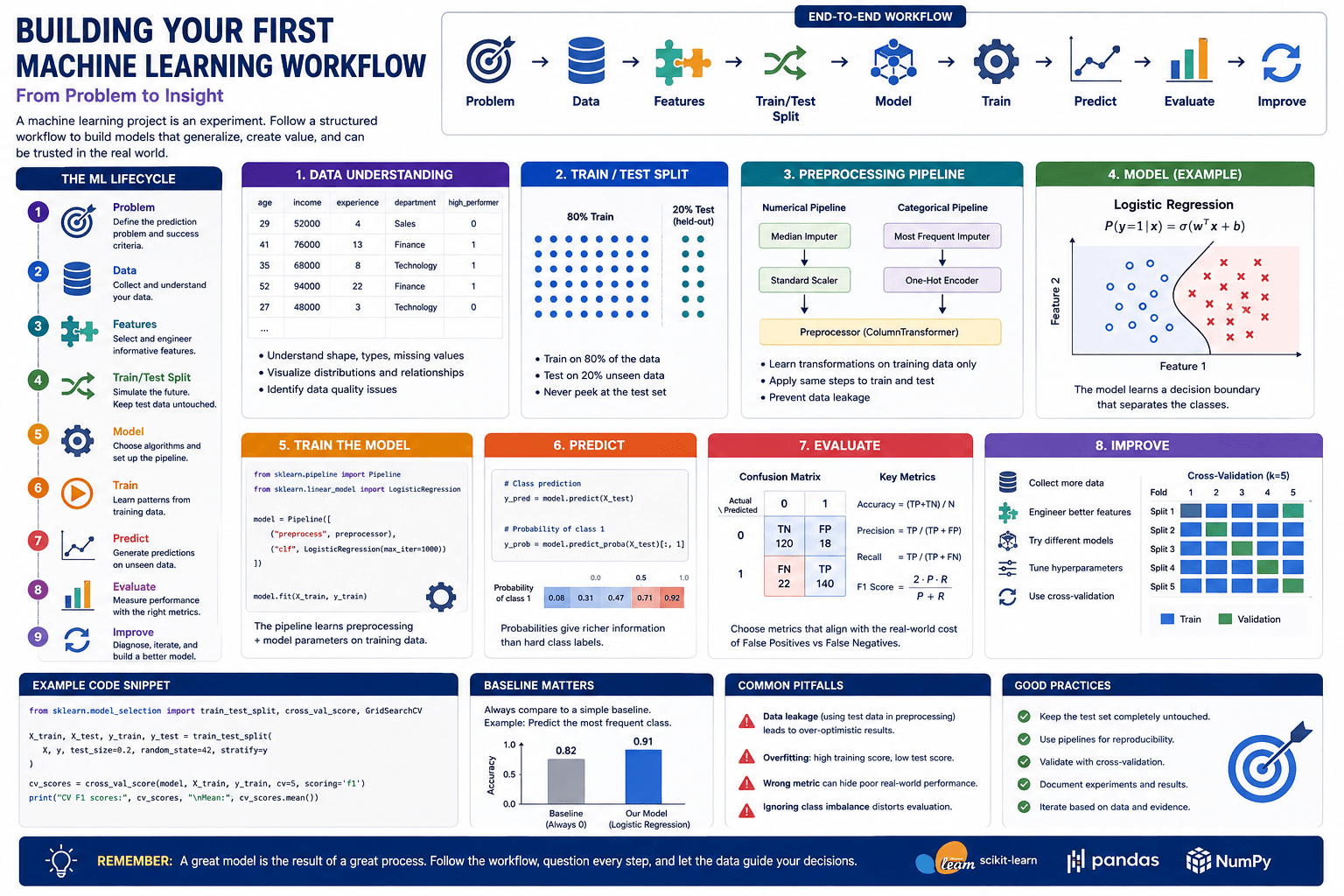
Problem → Data → Features → Train/Test Split → Preprocess → Model → Train → Predict → Evaluate → Improve

Begin with the Prediction Problem

Before choosing an algorithm, we need to define the task precisely. Machine learning begins not with a model but with a prediction problem.

Suppose we have historical information about employees containing variables such as age, income, years of experience, department, and performance score. If our objective is to predict a continuous performance score, we have a regression problem. If instead we want to predict whether an employee belongs to a category such as "high performer" or "standard performer," the task becomes classification.

This distinction determines the kinds of models and evaluation metrics that will be appropriate. Regression algorithms estimate continuous numerical quantities, while classification algorithms estimate classes or probabilities of class membership. Many other machine learning paradigms exist, including clustering, dimensionality reduction, anomaly detection, recommendation, and reinforcement learning, but supervised regression and classification provide an excellent foundation for understanding the complete workflow.

For this guide, we will use a classification problem. Imagine a dataset called employee_performance.csv containing historical observations:

import pandas as pd

df = pd.read_csv("employee_performance.csv")

print(df.head())
print(df.shape)
print(df.dtypes)

Suppose the target variable is high_performer, encoded as either 0 or 1. Our objective is therefore to estimate:

where $X$ represents the available features and $Y$ represents whether the employee belongs to the high-performance class.

This mathematical notation captures the essence of supervised learning: given what we know about an observation, how accurately can we estimate its unknown outcome?

Features and Targets: Defining What the Model Can Know

In supervised machine learning, the dataset is usually separated conceptually into a feature matrix $X$ and a target vector $y$.

If the dataset contains n observations and p features, we can write:

while the target vector is:

In practice, not every feature will necessarily be numerical, so the mathematical notation is an abstraction. Pandas allows us to preserve categorical variables until they are transformed later in the pipeline.

For example:

features = [
    "age",
    "income",
    "experience",
    "department"
]

X = df[features]
y = df["high_performer"]

print("Feature matrix:", X.shape)
print("Target vector:", y.shape)

Feature selection is not merely a programming decision. Every feature represents information the model will be permitted to use when making a prediction. A variable recorded after the outcome occurred may accidentally reveal the target. An identifier may allow the model to memorize observations without learning a useful pattern. A seemingly harmless proxy variable may encode sensitive or otherwise inappropriate information.

The central question is therefore not simply "Does this column improve accuracy?" It is "Would this information genuinely be available at the moment when the real-world prediction must be made?"

The Train/Test Split: Simulating the Future

A machine learning model should not be evaluated on the same observations it used for learning. If it were, a sufficiently flexible model could memorize the training data and appear highly accurate without learning patterns that generalize.

The standard solution is to reserve part of the dataset as unseen test data:

from sklearn.model_selection import train_test_split

X_train, X_test, y_train, y_test = train_test_split(
    X,
    y,
    test_size=0.20,
    random_state=42,
    stratify=y
)

Here, 80% of the observations are used for training and 20% are reserved for evaluation. random_state=42 makes the random split reproducible, while stratify=y helps preserve approximately the same class proportions in both subsets.

Conceptually, the test set represents the future.

The model is allowed to learn from:

but its ability to generalize is estimated using:

The test set should therefore remain untouched during model development whenever possible. Repeatedly examining test performance while adjusting the model gradually turns the test set into part of the development process, weakening its value as an independent estimate of generalization.

Preprocessing Must Learn from Training Data

Real datasets rarely arrive in model-ready form. Numerical columns may contain missing values, categorical features may require encoding, and variables may operate on dramatically different scales.

Suppose our numerical features are:

numeric_features = [
    "age",
    "income",
    "experience"
]

and our categorical feature is:

categorical_features = [
    "department"
]

A common numerical workflow might replace missing values with the median and standardize the resulting values. Standardization transforms a feature approximately according to:

where $\mu$ is the training mean and $\sigma$ is the training standard deviation.

Categorical variables can be imputed and then transformed using one-hot encoding. Scikit-learn allows both operations to be defined explicitly:

from sklearn.pipeline import Pipeline
from sklearn.impute import SimpleImputer
from sklearn.preprocessing import StandardScaler, OneHotEncoder
from sklearn.compose import ColumnTransformer

numeric_pipeline = Pipeline([
    ("imputer", SimpleImputer(strategy="median")),
    ("scaler", StandardScaler())
])

categorical_pipeline = Pipeline([
    ("imputer", SimpleImputer(strategy="most_frequent")),
    ("encoder", OneHotEncoder(handle_unknown="ignore"))
])

preprocessor = ColumnTransformer([
    ("numeric", numeric_pipeline, numeric_features),
    ("categorical", categorical_pipeline, categorical_features)
])

This may initially appear more elaborate than manually modifying the DataFrame. The advantage is methodological: preprocessing becomes part of the machine learning system itself.

When the pipeline is fitted on the training data, medians, means, standard deviations, and category mappings are learned only from that training subset. The same learned transformations are subsequently applied to unseen observations.

This protects the workflow from a subtle but extremely important problem: data leakage.

Data Leakage: When the Future Enters the Past

Data leakage occurs when information that should not be available during training influences the model. Leakage can produce exceptionally impressive evaluation scores while creating systems that fail dramatically in real-world deployment.

Imagine standardizing the complete dataset before performing the train/test split:

# Do not use this as a general workflow
X_scaled = scaler.fit_transform(X)

X_train, X_test, y_train, y_test = train_test_split(
    X_scaled,
    y,
    test_size=0.20,
    random_state=42
)

The transformation has already calculated statistics using every observation, including those that will later become test data. The model itself has not directly seen the test labels, but information from the test distribution has entered the training process.

A pipeline prevents this by fitting transformations only when fit() is called on the training subset.

Leakage can be much more serious than preprocessing contamination. Medical models may inadvertently receive information recorded after diagnosis. Financial models may contain variables generated after a default event. Predictive maintenance systems may include measurements collected after equipment failure. In each case, the model can appear remarkably intelligent because the answer is partially encoded in its inputs.

Establish a Baseline Before Building a Better Model

Before evaluating a sophisticated algorithm, we should ask how well an extremely simple strategy performs.

For classification, a baseline might always predict the most frequent class:

from sklearn.dummy import DummyClassifier

baseline = DummyClassifier(strategy="most_frequent")
baseline.fit(X_train[numeric_features], y_train)

baseline_accuracy = baseline.score(
    X_test[numeric_features],
    y_test
)

print("Baseline accuracy:", baseline_accuracy)

Suppose 82% of employees belong to the standard-performance category. A model that always predicts that class would achieve 82% accuracy while learning absolutely nothing.

If our machine learning model achieves 83%, describing it as "83% accurate" sounds impressive until we realize that it barely improves upon a trivial rule.

Baselines therefore provide context. They force us to answer the question that matters:

Is the model learning something useful?

Depending on the problem, a baseline might be a majority-class prediction, historical average, simple heuristic, linear model, or existing business process. Machine learning should demonstrate value relative to something meaningful rather than merely producing a numerical score.

Training the First Model

We can now attach a classifier to the preprocessing pipeline.

Logistic regression is an excellent first model because it is computationally efficient, widely understood, and often surprisingly competitive on structured datasets:

from sklearn.linear_model import LogisticRegression

model = Pipeline([
    ("preprocessor", preprocessor),
    ("classifier", LogisticRegression(max_iter=1000))
])

model.fit(X_train, y_train)

This single call performs several operations. Missing numerical values are imputed, numerical variables are standardized, categorical variables are encoded, and the transformed feature matrix is passed to logistic regression.

The important conceptual distinction is between fitting and transforming.

During training, the preprocessing components learn parameters from X_train, and the classifier learns parameters from the transformed training data. When new observations arrive, the pipeline uses the already learned preprocessing parameters before passing the transformed data to the trained model.

That separation makes the entire prediction workflow reproducible.

From Model to Prediction

Once the model has been fitted, predictions can be generated for the unseen test set:

y_pred = model.predict(X_test)

For many classification problems, however, predicted probabilities are even more informative:

y_prob = model.predict_proba(X_test)[:, 1]

A classifier may estimate that one observation has:

while another has:

If both are converted into class 1 using a threshold of 0.5, the final labels look identical even though the model's confidence differs substantially.

This distinction becomes important because the appropriate decision threshold depends on the application. In some domains, false positives are expensive; in others, missing a true positive is far more serious. Machine learning models often estimate probabilities, while humans and organizational policies determine how those probabilities should become decisions.

Accuracy Is Not Enough

For a binary classification problem, predictions can be summarized using a confusion matrix:

from sklearn.metrics import confusion_matrix

cm = confusion_matrix(y_test, y_pred)

print(cm)

The matrix separates predictions into true positives, true negatives, false positives, and false negatives. From these quantities, several metrics can be calculated.

Precision measures how often positive predictions are correct:

Recall measures how many actual positive cases the model successfully identifies:

The F1 score balances precision and recall through their harmonic mean:

Scikit-learn can calculate these automatically:

from sklearn.metrics import classification_report

print(
    classification_report(
        y_test,
        y_pred
    )
)

The appropriate metric depends on the consequences of errors. A disease-screening model may prioritize recall because missing a genuinely high-risk patient could be costly. A system automatically blocking legitimate financial transactions may place greater emphasis on controlling false positives.

Evaluation is therefore not purely mathematical. Metrics encode priorities.

Overfitting: When Learning Becomes Memorization

A model should capture patterns that extend beyond the observations used for training. When it learns the training data too specifically—including noise and accidental relationships—it overfits.

We can describe prediction error conceptually as:

The exact quantity and sign depend on the metric, but the principle is straightforward: a large difference between training and validation performance often signals that the model has learned patterns that do not transfer well.

Consider:

train_score = model.score(X_train, y_train)
test_score = model.score(X_test, y_test)

print("Training accuracy:", train_score)
print("Test accuracy:", test_score)

If training accuracy is 99% while test accuracy is 76%, increasing model complexity further is unlikely to solve the fundamental problem.

Possible responses include collecting more representative data, reducing model complexity, applying regularization, removing unstable features, improving feature engineering, or using better validation procedures.

This connects directly with Generalization & the Loss Landscape from The Science of AI. The objective of machine learning is not to minimize training error at any cost. It is to learn structures that remain useful outside the training sample.

Cross-Validation: Estimating Performance More Reliably

A single train/test split is useful, but the resulting performance estimate depends partly on which observations happened to enter each subset. When datasets are limited, this randomness can be substantial.

Cross-validation provides a more robust approach by repeatedly training and validating the model on different subsets of the training data.

In k-fold cross-validation, the training set is divided into k parts. The model trains on k-1 folds and validates on the remaining fold. The process repeats until each fold has served as validation data.

For example:

from sklearn.model_selection import cross_val_score

cv_scores = cross_val_score(
    model,
    X_train,
    y_train,
    cv=5,
    scoring="f1"
)

print("Fold scores:", cv_scores)
print("Mean F1:", cv_scores.mean())
print("Std F1:", cv_scores.std())

The mean provides an estimate of typical validation performance, while the variation across folds provides useful information about stability.

Because preprocessing is contained inside our pipeline, each cross-validation fold independently learns its preprocessing parameters from its own training portion. This is precisely why pipelines are so valuable: they preserve the experimental boundary automatically.

Improving the Model Systematically

Once a baseline and first model have been established, improvement should proceed as an experiment rather than a sequence of arbitrary algorithm changes.

We might compare logistic regression with a tree-based model:

from sklearn.ensemble import RandomForestClassifier

forest_model = Pipeline([
    ("preprocessor", preprocessor),
    ("classifier", RandomForestClassifier(
        n_estimators=300,
        random_state=42
    ))
])

We can then evaluate both models under the same cross-validation procedure. If the random forest performs better, we have evidence that nonlinear relationships or feature interactions may be useful.

Hyperparameters can also be tuned systematically. Rather than manually trying values, scikit-learn can search combinations under cross-validation:

from sklearn.model_selection import GridSearchCV

param_grid = {
    "classifier__C": [0.01, 0.1, 1, 10],
    "classifier__class_weight": [None, "balanced"]
}

search = GridSearchCV(
    model,
    param_grid=param_grid,
    cv=5,
    scoring="f1",
    n_jobs=-1
)

search.fit(X_train, y_train)

print(search.best_params_)
print(search.best_score_)

Notice that the test set has still not been used. Hyperparameter selection occurs entirely within the training data through cross-validation.

Only after the modeling decisions are finalized should the selected system be evaluated against the held-out test set.

The Pipeline Is the Model

A common conceptual mistake is to think that logistic regression, a random forest, or a neural network is the complete model.

In deployment, however, raw observations cannot usually be passed directly into the estimator. They must undergo exactly the same preprocessing used during training. Missing values must be handled consistently, categorical values encoded identically, numerical transformations preserved, and features presented in the expected form.

The actual predictive system is therefore:

not merely the estimator itself.

This is why the scikit-learn Pipeline abstraction is more than a programming convenience. It represents the true structure of the machine learning system.

A new observation can be processed safely:

new_employee = pd.DataFrame([{
    "age": 38,
    "income": 72000,
    "experience": 11,
    "department": "Technology"
}])

prediction = model.predict(new_employee)
probability = model.predict_proba(new_employee)[:, 1]

print("Prediction:", prediction[0])
print("Probability:", probability[0])

The same transformations learned during training are applied automatically before prediction.

Reproducibility and Experiment Tracking

The previous article in this series emphasized that reproducibility is a property of the entire computational workflow. Machine learning makes this even more important because an experiment now includes data selection, preprocessing, feature definitions, splitting strategy, algorithm choice, hyperparameters, random states, evaluation metrics, and software versions.

At minimum, a serious experiment should make these decisions explicit. As projects grow, dedicated experiment-tracking systems can record configurations, metrics, artifacts, and model versions automatically.

The objective is not bureaucratic documentation. It is the ability to answer questions such as: Which data trained this model? Which preprocessing was applied? Which hyperparameters produced this result? Which metric determined that it was better? Could we reproduce the model if the current environment disappeared?

If those questions cannot be answered, an apparently successful model may be difficult to trust, audit, improve, or deploy.

From Experiment to Machine Learning Workflow

We can now see why a machine learning project should be understood as a lifecycle rather than a single training operation.

The process begins by translating a real-world question into a measurable prediction task. Data is inspected and transformed into meaningful features. Training and evaluation data are separated before preprocessing parameters are learned. A baseline establishes what meaningful improvement looks like. Models are trained and evaluated using metrics appropriate to the consequences of their errors. Cross-validation provides more reliable estimates, while pipelines protect the experimental boundary and make transformations reproducible.

The workflow then becomes iterative. Evaluation reveals weaknesses, which lead to new hypotheses about data quality, features, model complexity, hyperparameters, or the formulation of the problem itself.

The central loop is therefore:

Define → Train → Evaluate → Diagnose → Improve → Re-evaluate

Machine learning expertise develops not from repeatedly calling .fit(), but from becoming increasingly skilled at reasoning through that loop.

Conclusion

Building your first machine learning workflow represents an important transition in the AI Skills Cookbook. In the previous guide, NumPy, Pandas, and visualization transformed raw observations into structured information. Here, those structures became the inputs to a predictive system.

The most important lesson is that model training occupies only one part of the process. Reliable machine learning requires careful problem formulation, defensible feature selection, strict separation between training and evaluation, leakage-resistant preprocessing, meaningful baselines, appropriate metrics, cross-validation, reproducible pipelines, and systematic experimentation.

A sophisticated algorithm cannot rescue an invalid experiment. Conversely, a relatively simple model embedded within a carefully designed workflow can provide remarkably strong and trustworthy results.

In the next guide, From Machine Learning to Deep Learning with PyTorch, we will move beneath abstractions such as model.fit() and examine how neural networks actually learn. Tensors will replace conventional feature matrices, predictions will emerge from forward passes, loss functions will quantify error, gradients will propagate backward through the network, and optimizers will update parameters iteratively.

That is where the workflow we have built here begins to reveal the computational machinery of modern deep learning.

Key Takeaways

• Machine learning begins with a well-defined prediction problem, not with selecting an algorithm.
• Supervised learning separates data into a feature matrix $X$ and target vector $y$.
• A train/test split creates an experimental approximation of how the model may perform on unseen future observations.
• Preprocessing parameters must be learned from training data to prevent data leakage.
• Scikit-learn pipelines combine preprocessing and estimation into a reproducible predictive system.
• A meaningful baseline establishes whether the machine learning model actually improves upon a simple alternative.
• Accuracy alone may conceal important differences between false positives and false negatives; metrics such as precision, recall, and F1 should reflect the real objective.
• Overfitting occurs when a model learns training-specific patterns that fail to generalize.
• Cross-validation provides a more robust estimate of model performance and supports model and hyperparameter selection.
• The test set should remain independent from iterative model development whenever possible.
• The complete predictive system includes preprocessing as well as the estimator—the pipeline is the model.
• Reliable machine learning depends as much on experimental design, reproducibility, and critical reasoning as it does on algorithms.