

If you find the content useful and wish to support our platform’s development, you can contribute any amount toward our production costs. Scan the UPI QR code for payment within India. Or use the Ko-fi link to process a secure payment via PayPal.
If you find the content useful and wish to support our platform’s development, you can contribute any amount toward our production costs. Scan the UPI QR code for payment within India. Or use the Ko-fi link to process a secure payment via PayPal.
In Module 1, you learned that statistics provides a systematic framework for collecting, organizing, analyzing, interpreting, and communicating data. Before meaningful conclusions can be drawn from any dataset, however, the data must first be summarized in a form that humans can understand. Real-world datasets often contain hundreds, thousands, or even millions of observations. Examining each individual value is neither practical nor informative. Descriptive Statistics provides the techniques needed to condense large datasets into meaningful numerical summaries and visual representations while preserving their essential characteristics.
Every data-driven discipline relies on descriptive statistics. Business analysts summarize sales performance before recommending strategic decisions, healthcare researchers examine patient measurements before evaluating treatments, and financial analysts study market trends before making investment recommendations. Similarly, data scientists perform descriptive analysis before building Machine Learning models because understanding the characteristics of a dataset is a prerequisite for reliable prediction. Throughout this module, you will learn how descriptive statistics transforms raw data into information that can be interpreted confidently and communicated effectively.
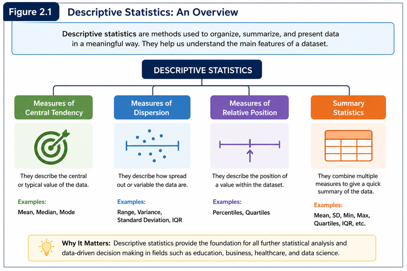
As shown in Figure 2.1, descriptive statistics acts as the bridge between raw observations and meaningful interpretation. Instead of attempting to memorize individual values, we summarize datasets using representative measures that describe the center, spread, and overall characteristics of the data. These summaries form the basis for later statistical procedures, including probability, hypothesis testing, correlation, regression, and predictive analytics.
After completing this module, you should be able to:
Imagine that an instructor wishes to compare the examination performance of twenty students enrolled in an introductory AI course. Although the complete dataset contains valuable information, reading every score individually makes it difficult to identify overall patterns. Questions such as "What is the typical score?", "How much do the scores vary?", and "Are there any unusually high or low values?" cannot be answered efficiently by simply inspecting the raw data. Descriptive statistics addresses this problem by reducing large collections of observations into a small number of informative measures.
This process can be viewed as a form of intelligent data compression. The original observations are retained, but their most important characteristics are represented by carefully selected summary statistics and graphical displays. Rather than replacing the dataset, descriptive statistics provides a concise description of its central tendency, variability, and distribution. These summaries allow analysts to understand the data quickly while preserving the information required for more advanced statistical analysis.
The remainder of this module introduces the principal numerical measures used to summarize data. We begin with the measures of central tendency, which describe the typical or representative value of a dataset. These measures—mean, median, and mode—form the foundation of descriptive statistical analysis and are among the most frequently reported statistics in research, business, and Artificial Intelligence.
When examining a dataset, one of the first questions we ask is, "What value best represents the data?" A dataset may contain many observations, but it is often useful to summarize them using a single value that describes the center or typical value of the distribution. Such measures are known as measures of central tendency. They provide a convenient way to compare datasets, identify overall performance, and communicate results clearly.
The three most widely used measures of central tendency are the mean, median, and mode. Each measure describes the center of a dataset from a different perspective and is appropriate under different circumstances. Throughout this module, you will learn not only how to calculate these measures but also when each one should be used and how to interpret the results correctly.
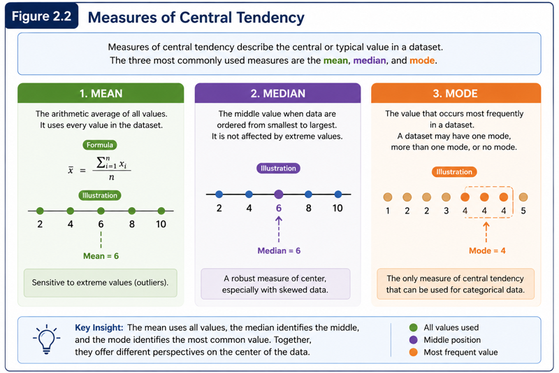
As illustrated in Figure 2.2, no single measure is universally "best." The nature of the dataset determines which measure provides the most meaningful summary. Later in this module, you will also see how unusual observations (outliers) can influence these measures differently.
The mean, commonly called the arithmetic average, is the most frequently reported measure of central tendency. It is obtained by adding all observations together and dividing by the total number of observations. Because every value contributes to the calculation, the mean incorporates all available information and is widely used in scientific research, business analytics, and Artificial Intelligence.
For a sample of size \(n\), the sample mean is calculated using the following formula:
\[ \bar{x}=\frac{\sum_{i=1}^{n}x_i}{n} \]| Symbol | Meaning |
|---|---|
| \(x_i\) | Individual observation |
| \(\sum x_i\) | Sum of all observations |
| \(n\) | Sample size |
| \(\bar{x}\) | Sample mean |
The notation introduced above follows standard statistical conventions and will be used consistently throughout this course. Becoming comfortable with these symbols now will make later topics, such as variance, standard deviation, confidence intervals, and regression, much easier to understand.
Five students obtained the following quiz scores:
| Student | Score |
|---|---|
| A | 68 |
| B | 72 |
| C | 75 |
| D | 81 |
| E | 84 |
Calculate the sample mean.
Step 1. Add all observations.
\[ 68+72+75+81+84=380 \]Step 2. Count the number of observations.
\[ n=5 \]Step 3. Apply the formula.
\[ \bar{x}=\frac{\sum x_i}{n} =\frac{380}{5} =76 \]The sample mean is
\[ \boxed{\bar{x}=76} \]The average quiz score for this group of students is 76 marks. Notice that the mean does not necessarily correspond to an actual student's score. Instead, it represents the balance point of the dataset and provides a single value that summarizes the overall performance of the group.
In the next part, we will examine the strengths and limitations of the mean, learn when it may produce misleading conclusions, and introduce the median, a measure of central tendency that is often more appropriate when datasets contain unusually large or small observations.
The mean is an extremely useful measure because it incorporates every observation in a dataset. Unlike the median and mode, every value contributes directly to its calculation. For this reason, the mean is widely used in scientific research, business reporting, educational assessment, and Machine Learning. However, because every observation influences the result, the mean can be affected substantially by unusually large or unusually small values, known as outliers. Later in this module we will examine outliers in detail and learn how they influence statistical summaries.
To begin developing the LearnerBox Student Learning Analytics Dataset, we will use a small teaching subset containing only the variables required for this lesson. As additional concepts are introduced throughout the course, this dataset will gradually expand to include more variables while remaining internally consistent.
| Student ID | Study Hours |
|---|---|
| ST001 | 4 |
| ST002 | 6 |
| ST003 | 5 |
| ST004 | 8 |
| ST005 | 7 |
| ST006 | 6 |
| ST007 | 9 |
| ST008 | 5 |
| ST009 | 7 |
| ST010 | 8 |
Using the teaching subset of Dataset A shown in Table 2.3, calculate the average number of study hours.
Step 1. Add all observations.
\[ 4+6+5+8+7+6+9+5+7+8=65 \]Step 2. Count the observations.
\[ n=10 \]Step 3. Apply the sample mean formula.
\[ \bar{x}=\frac{\sum x_i}{n} =\frac{65}{10} =6.5 \]The students in this teaching subset study an average of 6.5 hours during the period being measured. The mean summarizes the entire dataset using a single representative value, making it easier to compare this group with other groups of students. If another class had a mean of 8.0 study hours, we could immediately conclude that the second class spends more time studying on average.
The mean is most informative when the observations are numerical and the dataset does not contain extreme outliers that distort the average. Under these conditions, the mean makes efficient use of all available information and provides an excellent summary of the data. Consequently, it is the preferred measure of central tendency in many statistical analyses and is reported extensively in academic research.
The mean is commonly used for variables such as examination scores, age, height, weight, annual income (when not highly skewed), sales revenue, production output, and study hours. In later modules, you will also encounter the mean as a building block for probability distributions, confidence intervals, hypothesis tests, regression analysis, and Machine Learning algorithms.
The next measure of central tendency is the median. Unlike the mean, the median depends on the ordered position of observations rather than their numerical total, making it particularly useful when datasets contain unusually large or unusually small values.
Although the mean is the most widely reported measure of central tendency, it is not always the most appropriate summary of a dataset. When a dataset contains one or more unusually large or unusually small observations, the mean may be pulled away from the center of the distribution. In such situations, the median often provides a more representative measure of the typical value because it depends on the ordered position of the observations rather than on their numerical magnitude.
The median is the middle observation after all values have been arranged in ascending or descending order. If the number of observations is odd, the median is the single middle value. If the number of observations is even, the median is obtained by averaging the two middle observations.
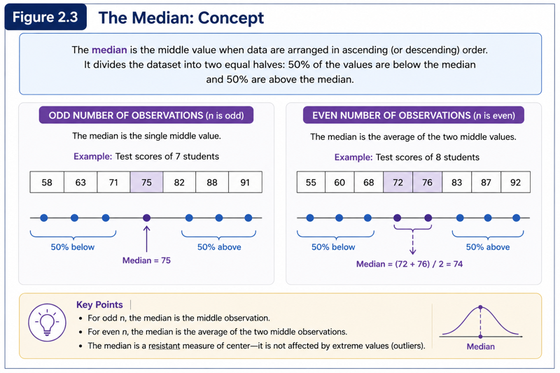
As shown in Figure 2.3, the median divides an ordered dataset into two equal halves. Approximately fifty percent of the observations lie below the median and fifty percent lie above it.
Using the teaching subset of Dataset A from Table 2.3, determine the median number of study hours.
Step 1. Arrange the observations in ascending order.
\[ 4,\;5,\;5,\;6,\;6,\;7,\;7,\;8,\;8,\;9 \]Step 2. Since there are ten observations, identify the two middle values.
\[ 6 \quad \text{and} \quad 7 \]Step 3. Calculate their average.
\[ \text{Median}=\frac{6+7}{2}=6.5 \]Half of the students in this teaching subset study 6.5 hours or less, while the remaining half study 6.5 hours or more. In this example, the mean and the median are identical because the observations are reasonably balanced and contain no extreme values.
Suppose another student who studied 30 hours is added to the dataset. Compare the effect on the mean and the median.
| Study Hours |
|---|
| 4 |
| 5 |
| 5 |
| 6 |
| 6 |
| 7 |
| 7 |
| 8 |
| 8 |
| 9 |
| 30 |
New mean:
\[ \bar{x}=\frac{95}{11}=8.64 \]New median:
\[ \boxed{\text{Median}=7} \]Adding a single unusually large observation increases the mean from 6.5 hours to 8.64 hours, whereas the median changes only slightly, from 6.5 hours to 7 hours. This example demonstrates that the median is considerably more resistant to extreme observations than the mean. Consequently, analysts often prefer the median when describing skewed datasets or data containing outliers.
The median is particularly useful for variables such as household income, property prices, waiting times, medical costs, and other measurements that frequently contain unusually high values. Many government agencies and international organizations report median income rather than mean income because a small number of extremely wealthy individuals can distort the average. In Artificial Intelligence and Data Analytics, the median is also used during data preprocessing because it provides a stable summary when datasets contain outliers or skewed distributions.
The third measure of central tendency is the mode, which identifies the most frequently occurring observation or category in a dataset. Unlike the mean and median, the mode can be applied to both numerical and categorical variables.
The mode is the value or category that occurs most frequently in a dataset. Unlike the mean and median, the mode is determined by frequency rather than by arithmetic calculations or ordered position. Consequently, it is the only measure of central tendency that can be applied to both numerical and categorical data. For categorical variables such as gender, blood group, product category, or preferred AI tool, the mode is often the only meaningful measure of central tendency.
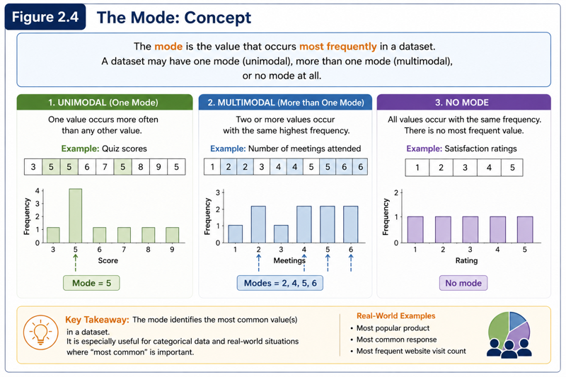
As shown in Figure 2.4, a dataset may have one mode (unimodal), two modes (bimodal), multiple modes (multimodal), or no mode when every observation occurs only once.
Using a teaching subset of Dataset A, determine the mode of the weekly study hours.
| Student ID | Study Hours |
|---|---|
| ST001 | 4 |
| ST002 | 6 |
| ST003 | 5 |
| ST004 | 8 |
| ST005 | 7 |
| ST006 | 6 |
| ST007 | 9 |
| ST008 | 5 |
| ST009 | 7 |
| ST010 | 8 |
Frequency of each value:
4 (1), 5 (2), 6 (2), 7 (2), 8 (2), 9 (1)
There is no unique mode because four values (5, 6, 7 and 8) share the highest frequency.
This example demonstrates that not every dataset has a single most frequent value. Reporting "the mode" without examining the frequency distribution can therefore be misleading. Whenever several values occur equally often, the analyst should report that the dataset is multimodal or has no unique mode.
A second teaching subset records the preferred AI tool used by ten students.
| Student ID | Preferred AI Tool |
|---|---|
| ST001 | ChatGPT |
| ST002 | ChatGPT |
| ST003 | Copilot |
| ST004 | ChatGPT |
| ST005 | Gemini |
| ST006 | ChatGPT |
| ST007 | Copilot |
| ST008 | ChatGPT |
| ST009 | Gemini |
| ST010 | ChatGPT |
ChatGPT appears 6 times, Copilot 2 times and Gemini 2 times.
The mode is ChatGPT.
Unlike the mean and median, the mode can summarize categorical information. For survey responses, customer preferences, medical diagnoses, or AI platform usage, the mode immediately identifies the most common category.
The mean, median and mode each describe the centre of a dataset from a different perspective. The mean uses every observation, the median identifies the middle position after ordering the data, and the mode identifies the most frequently occurring value or category. Rather than competing measures, they complement one another. Experienced analysts frequently report more than one measure because together they provide a richer description of the data.
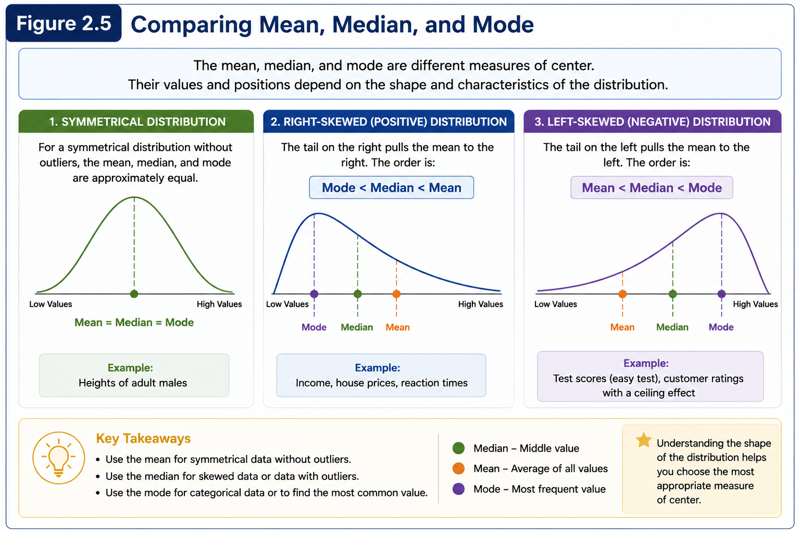
In the next part we move beyond measures of central tendency and introduce measures of dispersion, beginning with the variance. These statistics quantify how widely observations are spread around the centre of the dataset and are essential for understanding consistency, risk and variability.
Measures of central tendency describe the typical or representative value of a dataset, but they do not tell us how widely the observations are spread. Two datasets may have exactly the same mean while exhibiting very different levels of variability. One group of students may obtain examination scores that are all close to the class average, whereas another group may have scores ranging from very low to very high. Although the averages are identical, the two datasets clearly behave differently. Measures of dispersion quantify this variability and provide a more complete description of the data.
Understanding variability is essential in statistics because it reflects the consistency of the observations. Low variability indicates that the values are clustered closely around the center of the dataset, whereas high variability indicates that the observations are more widely dispersed. In AI and Machine Learning, variability also influences data preprocessing, anomaly detection, model evaluation, and feature engineering. For this reason, measures of dispersion are always interpreted alongside measures of central tendency.
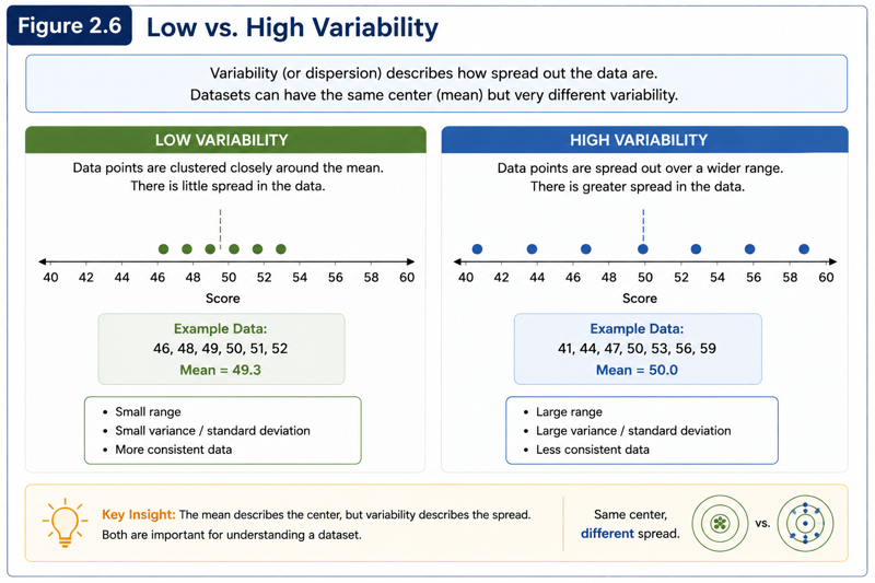
As illustrated in Figure 2.6, two datasets can share the same average while having completely different patterns of variation. Reporting only the mean would therefore provide an incomplete description of the data.
The variance measures the average squared distance of the observations from the mean. It is one of the most important measures of dispersion because it considers every observation in the dataset. The squaring process ensures that observations both above and below the mean contribute positively to the measure of variability.
For a sample, the variance is calculated using the following formula:
\[ s^2=\frac{\sum_{i=1}^{n}(x_i-\bar{x})^2}{n-1} \]| Symbol | Meaning |
|---|---|
| \(x_i\) | Individual observation |
| \(\bar{x}\) | Sample mean |
| \(n\) | Sample size |
| \(s^2\) | Sample variance |
Notice that the denominator is \(n-1\) rather than \(n\). This adjustment, known as Bessel's correction, produces an unbiased estimate of the population variance when calculations are based on a sample. A detailed explanation will be provided in Module 5 when sampling and statistical inference are introduced.
Using the teaching subset of Dataset A shown below, calculate the sample variance.
| Student ID | Study Hours |
|---|---|
| ST001 | 4 |
| ST002 | 6 |
| ST003 | 5 |
| ST004 | 8 |
| ST005 | 7 |
| ST006 | 6 |
| ST007 | 9 |
| ST008 | 5 |
| ST009 | 7 |
| ST010 | 8 |
The sample mean from Worked Example 2.2 was:
\[ \bar{x}=6.5 \]Step 1. Calculate each deviation from the mean.
Step 2. Square each deviation.
Step 3. Add the squared deviations.
\[ \sum (x_i-\bar{x})^2=22.50 \]Step 4. Divide by \(n-1\).
\[ s^2=\frac{22.50}{9}=2.50 \]The sample variance is 2.50 square hours. Because the unit of variance is squared, it is generally less intuitive to interpret directly. Nevertheless, variance is extremely important because it forms the mathematical foundation for many statistical techniques, including standard deviation, ANOVA, regression, and numerous Machine Learning algorithms.
The square root of the variance produces the standard deviation, a measure of dispersion expressed in the original units of the data. Because it is easier to interpret than the variance, the standard deviation is one of the most frequently reported descriptive statistics in research, business analytics, and Artificial Intelligence.
Although the variance is mathematically important, it is expressed in squared units, making it difficult to interpret directly. For example, if study time is measured in hours, the variance is measured in square hours. To overcome this limitation, statisticians use the standard deviation, which is simply the positive square root of the variance. Because the standard deviation is expressed in the original units of the data, it provides a much more intuitive measure of variability.
For a sample, the standard deviation is calculated using the following formula:
\[ s=\sqrt{\frac{\sum_{i=1}^{n}(x_i-\bar{x})^2}{n-1}} \]| Symbol | Meaning |
|---|---|
| \(x_i\) | Individual observation |
| \(\bar{x}\) | Sample mean |
| \(n\) | Sample size |
| \(s\) | Sample standard deviation |
The standard deviation is one of the most frequently reported descriptive statistics because it summarizes the typical distance of observations from the mean. Smaller values indicate greater consistency, whereas larger values indicate greater variability.
Using the variance calculated in Worked Example 2.7, determine the sample standard deviation.
From the previous example,
\[ s^2=2.50 \]Taking the positive square root,
\[ s=\sqrt{2.50}=1.5811 \]Rounded to two decimal places,
\[ \boxed{s=1.58\text{ hours}} \]The study hours typically vary by approximately 1.58 hours from the average value of 6.5 hours. Although individual students may study more or less than the average, the standard deviation provides a practical indication of the overall spread of the observations.
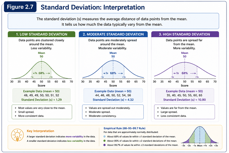
As illustrated in Figure 2.7, the standard deviation measures how tightly observations cluster around the mean. A small standard deviation indicates that most observations lie close to the center of the dataset, whereas a large standard deviation indicates greater dispersion.
Although understanding the manual calculations is essential, descriptive statistics are almost always computed using statistical software in professional practice. Microsoft Excel provides built-in functions such as AVERAGE(), VAR.S(), and STDEV.S(), while IBM SPSS Statistics can generate a complete descriptive statistics table with only a few commands. In both cases, software performs the arithmetic automatically, allowing analysts to focus on interpreting the results rather than carrying out repetitive calculations.
In later parts of this module, we will examine complete summary statistics generated by Excel and SPSS and learn how to interpret every value they report. Before doing so, however, we will introduce percentiles, which describe the relative position of observations within a dataset rather than simply its center or variability.
Measures of central tendency and measures of dispersion describe the overall characteristics of a dataset, but they do not indicate the relative position of an individual observation. In many practical situations, analysts wish to know where a particular value lies in comparison with the remaining observations. Percentiles answer this question by dividing an ordered dataset into one hundred equal parts and indicating the percentage of observations that fall below a specified value.
Percentiles are widely used in education, healthcare, psychology, finance, and business analytics. Examination scores are frequently reported as percentile ranks, medical growth charts are based on percentiles, and standardized tests often compare individual performance with that of a reference population. In Data Analytics, percentiles help identify unusually high or low observations and are commonly used when summarizing large datasets.
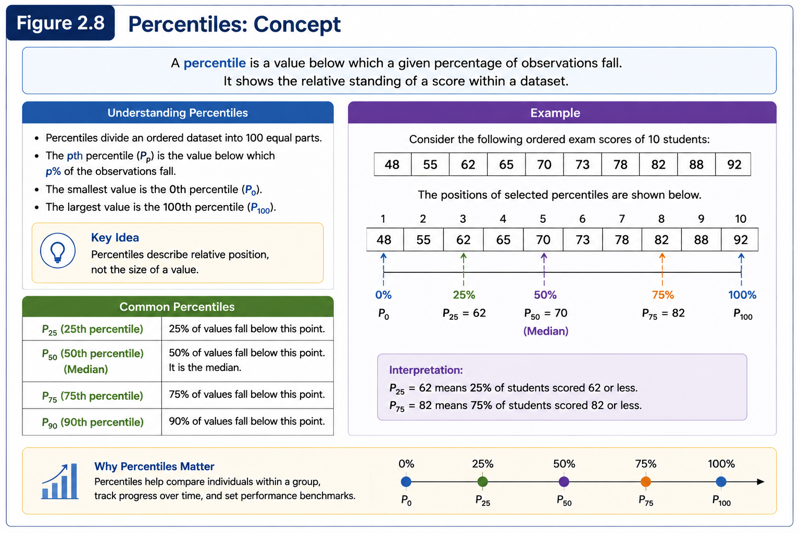
As illustrated in Figure 2.8, the 50th percentile is identical to the median because it divides the ordered dataset into two equal halves. Similarly, the 25th percentile and the 75th percentile play important roles in understanding the spread of the data and will later be used to identify outliers.
The following examination scores have already been arranged in ascending order.
| Student | Score |
|---|---|
| A | 55 |
| B | 60 |
| C | 64 |
| D | 68 |
| E | 72 |
| F | 75 |
| G | 78 |
| H | 82 |
| I | 88 |
| J | 94 |
Determine the median (50th percentile).
Since there are ten observations, the median is the average of the fifth and sixth values.
\[ \frac{72+75}{2}=73.5 \]Half of the students scored below 73.5 marks, while the remaining half scored above this value. Reporting the result as the 50th percentile emphasizes the student's relative position within the ordered distribution rather than simply identifying the middle value.
A special group of percentiles, known as quartiles, divides an ordered dataset into four equal parts. Quartiles are among the most frequently reported descriptive statistics because they summarize how observations are distributed across the dataset.
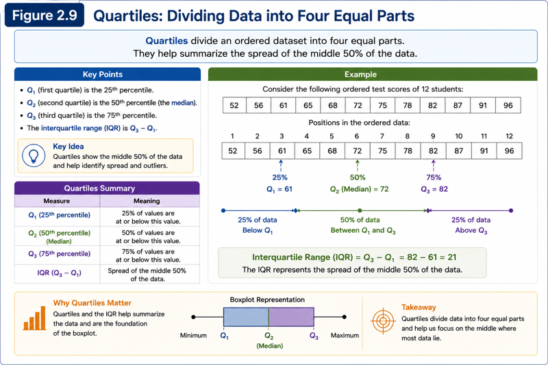
Quartiles provide valuable information about the distribution of observations and form the basis of the Interquartile Range (IQR), which will be introduced in the next part when discussing outliers and boxplots.
The next section builds directly upon these concepts by introducing the Interquartile Range (IQR) and demonstrating how quartiles can be used to identify unusually small or unusually large observations.
Not every observation in a dataset follows the general pattern of the remaining values. Occasionally, one or more observations are unusually small or unusually large when compared with the rest of the data. Such observations are known as outliers. Outliers are not necessarily errors; they may represent genuine but uncommon events. Nevertheless, because they can influence statistical summaries and analytical models, they should always be investigated carefully before any conclusions are drawn.
Outliers may arise for several reasons. They can result from measurement or data-entry errors, natural variation within the population, or genuinely exceptional cases. For example, a student who studies considerably longer than everyone else, an unusually expensive house in a property dataset, or an exceptionally high medical bill may all appear as outliers. Identifying these observations is an important part of exploratory data analysis and is routinely performed before developing statistical or Machine Learning models.
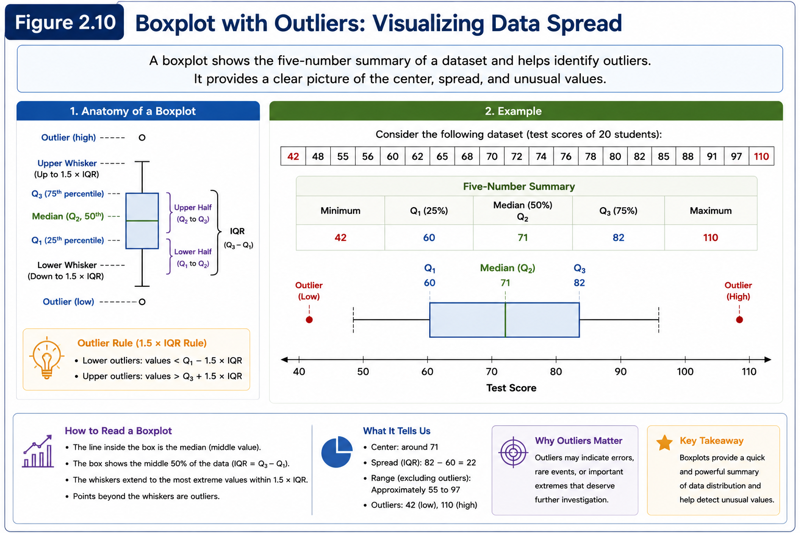
As illustrated in Figure 2.10, one of the most effective methods for identifying outliers is the boxplot. Although boxplots will be explored in greater detail in Module 3, understanding how they relate to quartiles and the Interquartile Range is useful at this stage.
The Interquartile Range (IQR) measures the spread of the middle fifty percent of the observations. Unlike the variance and standard deviation, the IQR is based on quartiles rather than every observation. Consequently, it is much less affected by extreme values and is particularly useful for skewed datasets.
The IQR is calculated using the following expression:
\[ IQR = Q_3 - Q_1 \]Using the ordered examination scores from Table 2.10, suppose:
\[ Q_1=62,\qquad Q_3=84 \]Calculate the Interquartile Range.
Apply the formula:
\[ IQR=Q_3-Q_1 \] \[ IQR=84-62=22 \]The middle fifty percent of the examination scores are spread across 22 marks. Because the IQR ignores the lowest and highest observations, it provides a robust measure of variability even when extreme values are present.
A commonly used rule identifies potential outliers by extending 1.5 times the IQR beyond the first and third quartiles.
The lower boundary is
\[ Q_1-1.5(IQR) \]and the upper boundary is
\[ Q_3+1.5(IQR) \]Any observation falling outside these limits is considered a potential outlier and should be investigated further.
Using the previous example,
\[ Q_1=62,\qquad Q_3=84,\qquad IQR=22 \]Lower boundary:
\[ 62-1.5(22)=29 \]Upper boundary:
\[ 84+1.5(22)=117 \]Suppose an additional score of 125 is recorded.
Since
\[ 125>117 \]the value is identified as a potential outlier.
The descriptive statistics introduced in this module can now be combined to provide a comprehensive summary of a dataset. In the next part, we will examine how software such as Microsoft Excel and IBM SPSS Statistics generates complete summary tables and how those results should be interpreted.
Up to this point, each descriptive statistic has been calculated and interpreted individually. In practice, however, analysts rarely compute the mean, median, standard deviation, quartiles, and other descriptive measures one at a time. Instead, statistical software generates a comprehensive summary table that presents the most important descriptive statistics together. Learning to interpret these summary tables is an essential skill because they are widely used in research papers, business reports, healthcare studies, government publications, and AI-driven analytics.
A summary statistics table provides a concise overview of the characteristics of a dataset. By examining a single table, an analyst can determine the number of observations, the average value, the variability of the data, the minimum and maximum values, and the overall distribution of the observations. These summaries often provide enough information to identify patterns, detect unusual values, and decide whether more advanced statistical analyses are appropriate.
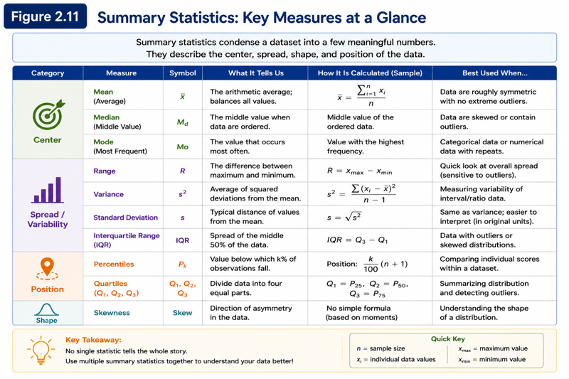
As illustrated in Figure 2.11, summary statistics bring together several descriptive measures into a single, easy-to-read format. Rather than interpreting each statistic in isolation, analysts examine them collectively to gain a comprehensive understanding of the dataset.
Suppose Microsoft Excel or IBM SPSS Statistics produces the following descriptive summary for the Study Hours variable.
| Statistic | Value |
|---|---|
| Sample Size (N) | 10 |
| Mean | 6.50 |
| Median | 6.50 |
| Standard Deviation | 1.58 |
| Minimum | 4 |
| Maximum | 9 |
The dataset contains ten observations. Students study an average of 6.5 hours, with the middle observation also equal to 6.5 hours. The standard deviation of 1.58 hours indicates moderate variability, while the minimum and maximum values suggest that no unusually extreme observations are present in this teaching subset.
Microsoft Excel provides several methods for calculating descriptive statistics. Individual statistics can be calculated using built-in functions such as AVERAGE(), MEDIAN(), MODE.SNGL(), VAR.S(), and STDEV.S(). For larger datasets, the Data Analysis ToolPak can generate a complete descriptive statistics table containing many measures simultaneously.
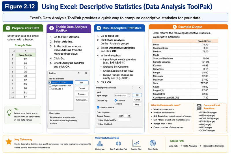
When using Excel, analysts should verify that the correct data range has been selected and should carefully distinguish between sample functions (for example, STDEV.S) and population functions (such as STDEV.P). Selecting the appropriate function depends upon whether the available data represent a sample or an entire population.
IBM SPSS Statistics automates descriptive statistical analysis through the Descriptive Statistics procedures. After selecting the required variables, SPSS produces professionally formatted output tables that include measures of central tendency, measures of dispersion, and additional descriptive statistics.
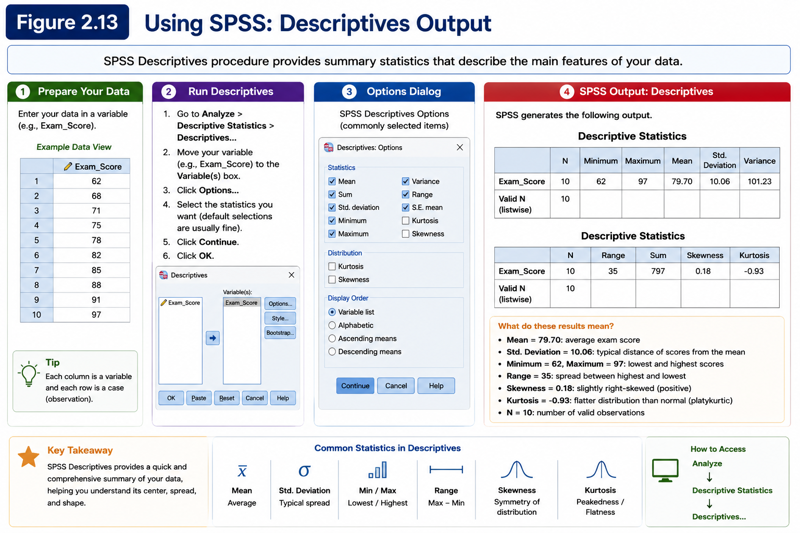
Because SPSS automatically performs all calculations, the analyst's primary responsibility is to interpret the output correctly. Understanding the concepts developed throughout this module ensures that the software results can be evaluated critically rather than accepted without question.
The following exercises provide an opportunity to apply the descriptive statistical techniques introduced throughout this module. Some questions require manual calculations, while others encourage you to verify your answers using Microsoft Excel or IBM SPSS Statistics. Remember that the objective is not merely to obtain the correct numerical answer, but also to interpret the statistical results within the context of the problem.
This module introduced the fundamental descriptive statistical techniques used to summarize and interpret numerical data. Beginning with measures of central tendency, you learned how the mean, median, and mode each describe the centre of a dataset from different perspectives. You then explored measures of dispersion, including the variance and standard deviation, to understand how observations vary around the average. Building upon these concepts, you examined percentiles, quartiles, the Interquartile Range, and methods for identifying potential outliers. Finally, you learned how descriptive statistics are generated and interpreted using Microsoft Excel and IBM SPSS Statistics, reinforcing the principle that software should support statistical reasoning rather than replace it. These concepts provide the numerical foundation for the more advanced analytical techniques introduced in the remaining modules.
Take a short Quiz and find your score. You can always come back to this page and go through the content again!